The BRDF
Ultimately, physically based rendering comes down to computing the radiance entering the camera along some set of view rays. Using the notation for incoming radiance introduced in Section 8.1.1, for a given view ray the quantity we need to compute is $L_i(c, v)$, where $c$ is the camera position and $v$ is the direction along the view ray. We use $v$ due to two notation conventions. First, the direction vector in $L_i()$ always points away from the given point, which in this case is the camera location. Second, the view vector $v$ always points toward the camera.
In rendering, scenes are typically modeled as collections of objects with media in between them (the word “media” actually comes from the Latin word for “in the middle” or “in between”). Often the medium in question is a moderate amount of relatively clean air, which does not noticeably affect the ray’s radiance and can thus be ignored for rendering purposes. Sometimes the ray may travel through a medium that does affect its radiance appreciably via absorption or scattering. Such media are called participating media since they participate in the light’s transport through the scene. Participating media will be covered in detail in Chapter 14. In this chapter we assume that there are no participating media present, so the radiance entering the camera is equal to the radiance leaving the closest object surface in the direction of the camera: \(L_i(c, v) = L_o(p, v)\) where $p$ is the intersection of the view ray with the closest object surface.
Following Equation above, our new goal is to calculate $L_o(p, v)$. This calculation is a physically based version of the shading model evaluation discussed in Section 5.1. Sometimes radiance is directly emitted by the surface. More often, radiance leaving the surface originated from elsewhere and is reflected by the surface into the view ray, via the physical interactions described in Section 9.1. In this chapter we leave aside the cases of transparency (Section 5.5 and Section 14.5.2) and global subsurface scattering (Section 14.6). In other words, we focus on local reflectance phenomena, which redirect light hitting the currently shaded point back outward. These phenomena include surface reflection as well as local subsurface scattering, and depend on only the incoming light direction $l$ and the outgoing view direction $v$. Local reflectance is quantified by the bidirectional reflectance distribution function (BRDF), denoted as $f(l, v)$.
In its original derivation the BRDF was defined for uniform surfaces. That is, the BRDF was assumed to be the same over the surface. However, objects in the real world (and in rendered scenes) rarely have uniform material properties over their surface. Even an object that is composed of a single material, e.g., a statue made of silver, will have scratches, tarnished spots, stains, and other variations that cause its visual properties to change from one surface point to the next. Technically, a function that captures BRDF variation based on spatial location is called a spatially varying BRDF (SVBRDF) or spatial BRDF (SBRDF). However, this case is so prevalent in practice that the shorter term BRDF is often used and implicitly assumed to depend on surface location.
The incoming and outgoing directions each have two degrees of freedom. A frequently used parameterization involves two angles: elevation $\theta$ relative to the surface normal $n$ and azimuth (horizontal rotation) $\phi$ about $n$. In the general case, the BRDF is a function of four scalar variables. Isotropic BRDFs are an important special case. Such BRDFs remain the same when the incoming and outgoing directions are rotated around the surface normal, keeping the same relative angles between them. Figure 9.17 shows the variables used in both cases. Isotropic BRDFs are functions of three scalar variables, since only a single angle $\phi$ between the light’s and camera’s rotation is needed. What this means is that if a uniform isotropic material is placed on a turntable and rotated, it will appear the same for all rotation angles, given a fixed light and camera.
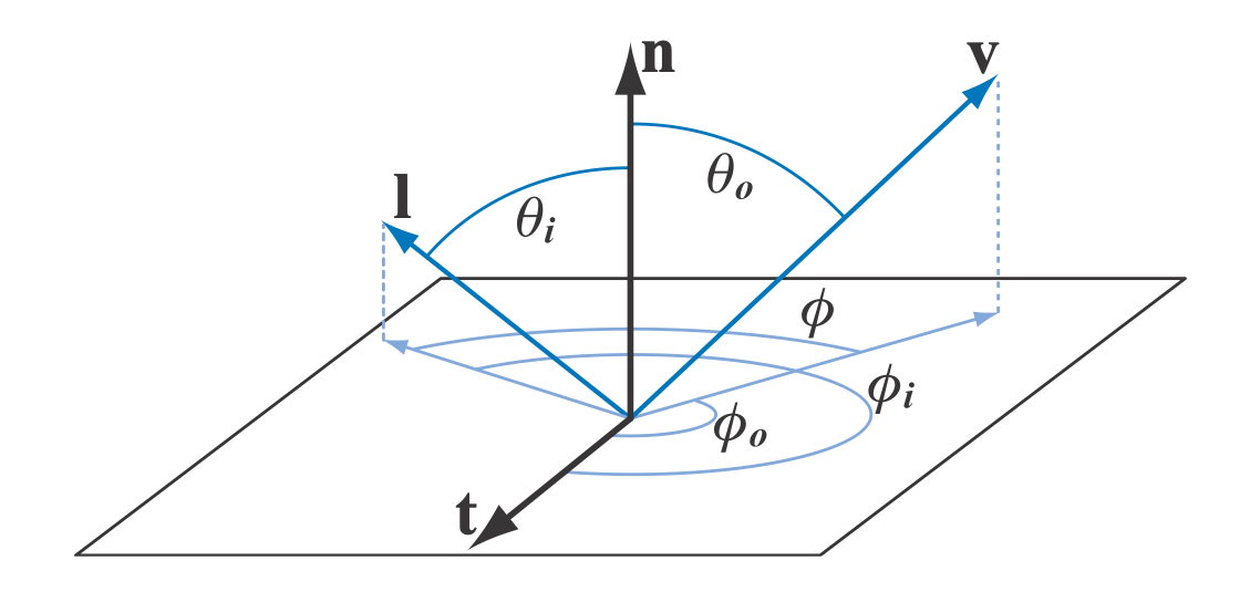
Figure 9.17: The BRDF. Azimuth angles $\phi_i$ and $\phi_o$ are given with respect to a given tangent vector $t$. The relative azimuth angle $\phi$, used for isotropic BRDFs instead of $\phi_i$ and $\phi_o$, does not require a reference tangent vector.
Since we ignore phenomena such as fluorescence and phosphorescence, we can assume that incoming light of a given wavelength is reflected at the same wavelength. The amount of light reflected can vary based on the wavelength, which can be modeled in one of two ways. Either the wavelength is treated as an additional input variable to the BRDF, or the BRDF is treated as returning a spectrally distributed value. While the first approach is sometimes used in offline rendering , in real-time rendering the second approach is always used. Since real-time renderers represent spectral distributions as RGB triples, this simply means that the BRDF returns an RGB value.
To compute $L_o(p, v)$, we incorporate the BRDF into the reflectance equation:
\[L_o(p, v) = \int_{l \in \Omega} f(l, v) L_i(p, l) (n\cdot l) dl\]The $l\in \Omega$ subscript on the integral sign means that integration is performed over $l$ vectors that lie in the unit hemisphere above the surface (centered on the surface normal $n$). Note that $l$ is swept continuously over the hemisphere of incoming directions?it is not a specific “light source direction.” The idea is that any incoming direction can (and usually will) have some radiance associated with it. We use $dl$ to denote the differential solid angle around $l$ (solid angles are discussed in Section 8.1.1).
In summary, the reflectance equation shows that outgoing radiance equals the integral (over $l$ in $\Omega$) of incoming radiance times the BRDF times the dot product between $n$ and $l$.
For brevity, for the rest of the chapter we will omit the surface point $p$ from $L_i()$, $L_o()$, and the reflectance equation: \(L_o(v) = \int_{l \in \Omega} f(l, v) L_i(l) (n\cdot l) dl\)
When computing the reflectance equation, the hemisphere is often parameterized using spherical coordinates $\phi$ and $\theta$. For this parameterization, the differential solid angle $dl$ is equal to $ \sin \theta_i d\theta_i d\phi_i$ . Using this parameterization, a double-integral form of Equation above can be derived, which uses spherical coordinates (recall that $(n\cdot l) = \cos \theta_i$): \(L_o(\theta_o, \phi_o) = \int_{\phi_i=0}^{2\pi} \int_{\theta_i=0}^{\pi/2} f(\theta_i, \phi_i, \theta_o, \phi_o) L_i(\theta_i, \phi_i)\cos\theta_i\sin\theta_id\theta_id\phi_i\) The angles $\theta_i$ , $\phi_i$ , $\theta_o$ , and $\phi_o$ are shown in Firgure 9.17.
In some cases it is convenient to use a slightly different parameterization, with the cosines of the elevation angles $\mu_i = \cos \theta_i$ and $\mu_o = \cos \theta_o$ as variables rather than the angles $\theta_i$ and $\theta_o$ themselves. For this parameterization, the differential solid angle $dl$ is equal to $d\mu_i d\phi_i$. Using the $(\mu, \phi)$ parameterization yields the following integral form: \(L_o(\mu_o, \phi_o) = \int_{\phi_i=0}^{2\pi} \int_{\mu_i= 0}^{1} f(\mu_i, \phi_i, \mu_o, \phi_o) L_i(\mu_i, \phi_i)\mu_id\mu_id\phi_i\)
The BRDF is defined only in cases where both the light and view directions are above the surface. The case where the light direction is under the surface can be avoided by either multiplying the BRDF by zero or not evaluating the BRDF for such directions in the first place. But what about view directions under the surface, in other words where the dot product $n \cdot v$ is negative? Theoretically this case should never occur. The surface would be facing away from the camera and would thus be invisible. However, interpolated vertex normals and normal mapping, both common in real-time applications, can create such situations in practice. Evaluation of the BRDF for view directions under the surface can be avoided by clamping $n \cdot v$ to 0 or using its absolute value, but both approaches can result in artifacts. The Frostbite engine uses the absolute value of $n \cdot v$ plus a small number (0.00001) to avoid divides by zero . Another possible approach is a “soft clamp,” which gradually goes to zero as the angle between n and v increases past $90^\circ$.
The laws of physics impose two constraints on any BRDF. The first constraint is Helmholtz reciprocity, which means that the input and output angles can be switched and the function value will be the same: \(f(l,v) = f(v,l)\)
In practice, BRDFs used in rendering often violate Helmholtz reciprocity without noticeable artifacts, except for offline rendering algorithms that specifically require reciprocity, such as bidirectional path tracing. However, it is a useful tool to use when determining if a BRDF is physically plausible.
The second constraint is conservation of energy?the outgoing energy cannot be greater than the incoming energy (not counting glowing surfaces that emit light, which are handled as a special case). Offline rendering algorithms such as path tracing require energy conservation to ensure convergence. For real-time rendering, exact energy conservation is not necessary, but approximate energy conservation is important. A surface rendered with a BRDF that significantly violates energy conservation would be too bright, and so may look unrealistic.
The directional-hemispherical reflectance R(l) is a function related to the BRDF. It can be used to measure to what degree a BRDF is energy conserving. Despite its somewhat daunting name, the directional-hemispherical reflectance is a simple concept. It measures the amount of light coming from a given direction that is reflected at all, into any outgoing direction in the hemisphere around the surface normal. Essentially, it measures energy loss for a given incoming direction. The input to this function is the incoming direction vector l, and its definition is presented here: \(R(l) = \int_{v \in \Omega} f(l, v) (n\cdot v) dv\) Note that here $v$, like $l$ in the reflectance equation, is swept over the entire hemisphere and does not represent a singular viewing direction.
A similar but in some sense opposite function, hemispherical-directional reflectance $R(v)$ can be similarly defined: \(R(v) = \int_{l \in \Omega} f(l, v) (n\cdot l) dl\)
If the BRDF is reciprocal, then the hemispherical-directional reflectance and the directional-hemispherical reflectance are equal and the same function can be used to compute either one. Directional albedo can be used as a blanket term for both reflectances in cases where they are used interchangeably.
The value of the directional-hemispherical reflectance $R(l)$ must always be in the range [0, 1], as a result of energy conservation. A reflectance value of 0 represents a case where all the incoming light is absorbed or otherwise lost. If all the light is reflected, the reflectance will be 1. In most cases it will be somewhere between these two values. Like the BRDF, the values of $R(l)$ vary with wavelength, so it is represented as an RGB vector for rendering purposes. Since each component (red, green, and blue) is restricted to the range [0, 1], a value of $R(l)$ can be thought of as a simple color.
Note that this restriction does not apply to the values of the BRDF. As a distribution function, the BRDF can have arbitrarily high values in certain directions (such as the center of a highlight) if the distribution it describes is highly nonuniform. The requirement for a BRDF to be energy conserving is that $R(l)$ be no greater than one for all possible values of $l$.
The simplest possible BRDF is Lambertian, which corresponds to the Lambertian shading model briefly discussed in Section 5.2. The Lambertian BRDF has a constant value. The well-known $(n \cdot l)$ factor that distinguishes Lambertian shading is not part of the BRDF but rather part of the rendering equation. Despite its simplicity, the Lambertian BRDF is often used in real-time rendering to represent local subsurface scattering (though it is being supplanted by more accurate models, as discussed in Section 9.9). The directional-hemispherical reflectance of a Lambertian surface is also a constant. Evaluating Equation 9.8 for a constant value of $f(l, v)$ yields the following value for the directional-hemispherical reflectance as a function of the BRDF: \(R(l) = \pi f(l, v)\)
The constant reflectance value of a Lambertian BRDF is typically referred to as the diffuse color $c_{diff}$ or the albedo $\rho$. In this chapter, to emphasize the connection with subsurface scattering, we will refer to this quantity as the subsurface albedo $\rho_{ss}$. The subsurface albedo is discussed in detail in Section 9.9.1. The BRDF from Equation above gives the following result: \(f(l, v) = \frac{\rho_{ss}}{\pi}\) The $1/\pi$ factor is caused by the fact that integrating a cosine factor over the hemisphere yields a value of $\pi$. Such factors are often seen in BRDFs.
Albedo is a term in planetary physics used to describe the reflective ability of a celestial body. Its mathematical definition is the ratio of reflected radiation to incident radiation, and it is a dimensionless quantity. Reflectance, on the other hand, is used to represent the ratio of reflected radiation to incident radiation for a specific wavelength of light. When only diffuse reflection exists and there is no specular reflection, albedo equals diffuse, with a value ranging from 0 to 1.
One way to understand a BRDF is to visualize it with the input direction held constant. See Figure 9.18. For a given direction of incoming light, the BRDF’s values are displayed for all outgoing directions. The spherical part around the point of intersection is the diffuse component, since outgoing radiance has an equal chance of reflecting in any direction. The ellipsoidal piece is the specular lobe. Naturally, such lobes are in the reflection direction from the incoming light, with the thickness of the lobe corresponding to the fuzziness of the reflection. By the principle of reciprocity, these same visualizations can also be thought of as how much each different incoming light direction contributes to a single outgoing direction.
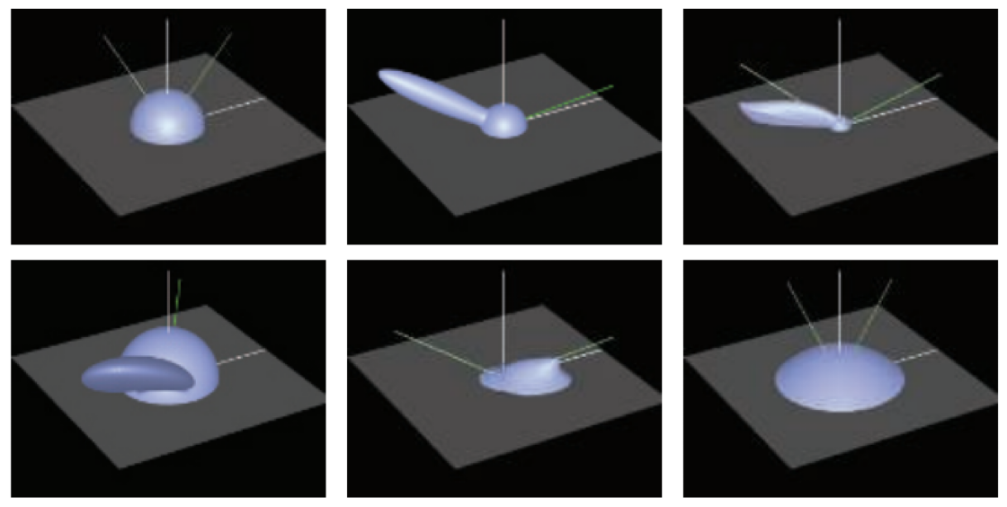
Figure 9.18. Example BRDFs. The solid green line coming from the right of each figure is the incoming light direction, and the dashed green and white line is the ideal reflection direction. In the top row, the left figure shows a Lambertian BRDF (a simple hemisphere). The middle figure shows Blinn-Phong highlighting added to the Lambertian term. The right figure shows the Cook-Torrance BRDF . Note how the specular highlight is not strongest in the reflection direction. In the bottom row, the left figure shows a close-up of Ward’s anisotropic model. In this case, the effect is to tilt the specular lobe. The middle figure shows the Hapke/Lommel-Seeliger “lunar surface” BRDF , which has strong retroreflection. The right figure shows Lommel-Seeliger scattering, in which dusty surfaces scatter light toward grazing angles.