Shadow Mapping
A common z-buffer-based renderer could be used to generate shadows quickly on arbitrary objects. The idea is to render the scene, using the z-buffer, from the position of the light source that is to cast shadows. Whatever the light “sees” is illuminated, the rest is in shadow. When this image is generated, only z-buffering is required. Lighting, texturing, and writing values into the color buffer can be turned off.
Each pixel in the z-buffer now contains the z-depth of the object closest to the light source. We call the entire contents of the z-buffer the shadow map, also sometimes known as the shadow depth map or shadow buffer. To use the shadow map, the scene is rendered a second time, but this time with respect to the viewer. As each drawing primitive is rendered, its location at each pixel is compared to the shadow map. If a rendered point is farther away from the light source than the corresponding value in the shadow map, that point is in shadow, otherwise it is not. This technique is implemented by using texture mapping. Shadow mapping is a popular algorithm because it is relatively predictable. The cost of building the shadow map is roughly linear with the number of rendered primitives, and access time is constant.
The shadow map can be generated once and reused each frame for scenes where the light and objects are not moving, such as for computer-aided design.
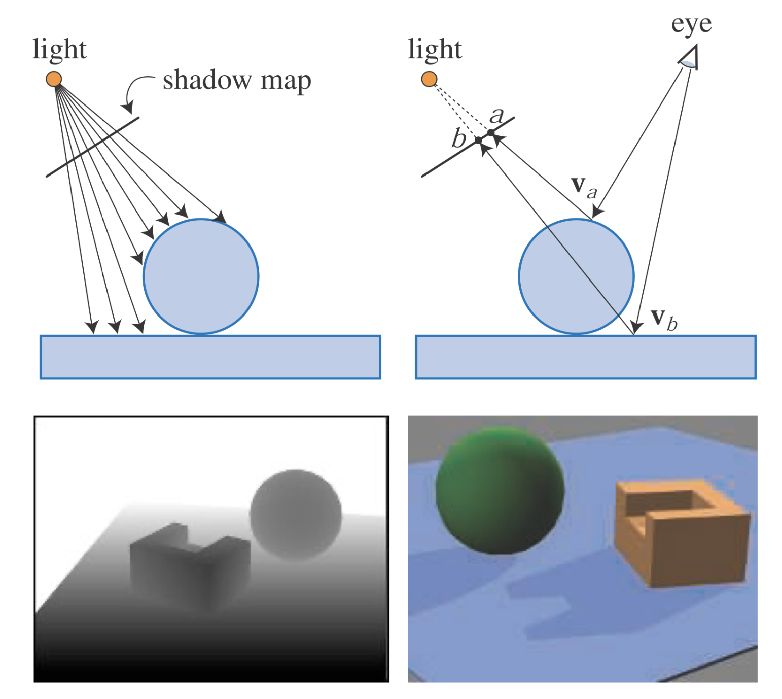
Shadow mapping. On the top left, a shadow map is formed by storing the depths to the surfaces in view. On the top right, the eye is shown looking at two locations. The sphere is seen at point $v_a$, and this point is found to be located at texel $a$ on the shadow map. The depth stored there is not (much) less than point $v_a$ is from the light, so the point is illuminated. The rectangle hit at point $v_b$ is (much) farther away from the light than the depth stored at texel $b$, and so is in shadow. On the bottom left is the view of a scene from the light’s perspective, with white being farther away. On the bottom right is the scene rendered with this shadow map.
When a single z-buffer is generated, the light can “look” in only a particular direction, like a camera. For a distant directional light such as the sun, the light’s view is set to encompass all objects casting shadows into the viewing volume that the eye sees. The light uses an orthographic projection, and its view needs to be made wide and high enough in x and y to view this set of objects. Local light sources need similar adjustments, as possible. If the local light is far enough away from the shadow-casting objects, a single view frustum may be sufficient to encompass all of these. Alternately, if the local light is a spotlight, it has a natural frustum associated with it, with everything outside its frustum considered not illuminated.
If the local light source is inside a scene and is surrounded by shadow-casters, a typical solution is to use a six-view cube, similar to cubic environment mapping. These are called omnidirectional shadow maps. The main challenge for omnidirectional maps is avoiding artifacts along the seams where two separate maps meet. Forsyth presents a general multi-frustum partitioning scheme for omnidirectional lights that also provides more shadow map resolution where needed. Crytek sets the resolution of each of the six views for a point light based on the screen-space coverage of each view’s projected frustum, with all maps stored in a texture atlas.
Not all objects in the scene need to be rendered into the light’s view volume. First, only objects that can cast shadows need to be rendered. For example, if it is known that the ground can only receive shadows and not cast one, then it does not have to be rendered into the shadow map.
Shadow casters are by definition those inside the light’s view frustum. This frustum can be augmented or tightened in several ways, allowing us to safely disregard some shadow casters. Think of the set of shadow receivers visible to the eye. This set of objects is within some maximum distance along the light’s view direction. Anything beyond this distance cannot cast a shadow on the visible receivers. Similarly, the set of visible receivers may well be smaller than the light’s original x and y view bounds. Another example is that if the light source is inside the eye’s view frustum, no object outside this additional frustum can cast a shadow on a receiver. Another example is that if the light source is inside the eye’s view frustum, no object outside this additional frustum can cast a shadow on a receiver. Rendering only relevant objects not only can save time rendering, but can also reduce the size required for the light’s frustum and so increase the effective resolution of the shadow map, thus improving quality. In addition, it helps if the light frustum’s near plane is as far away from the light as possible, and if the far plane is as close as possible. Doing so increases the effective precision of the z-buffer.
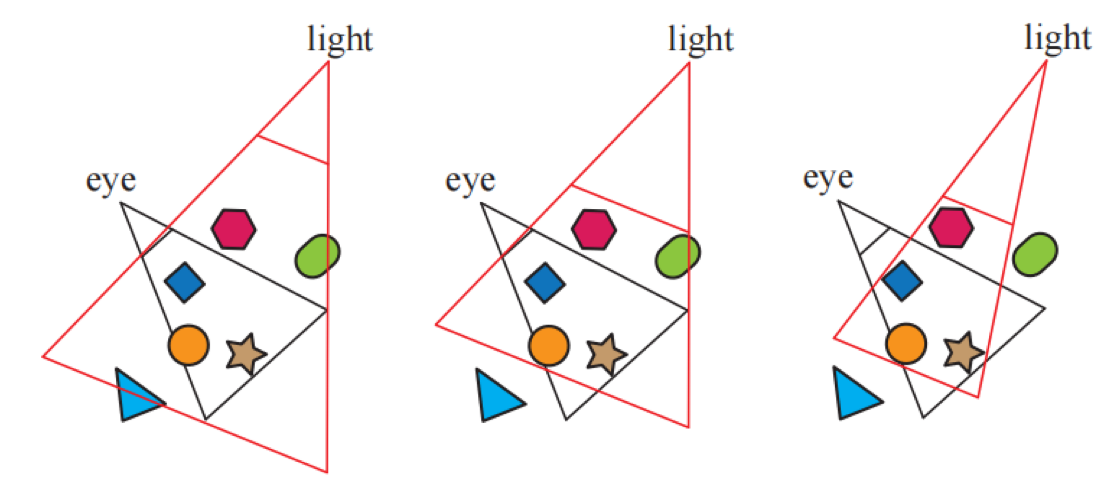
On the left, the light’s view encompasses the eye’s frustum. In the middle, the light’s far plane is pulled in to include only visible receivers, so culling the triangle as a caster; the near plane is also adjusted. On the right, the light’s frustum sides are made to bound the visible receivers, culling the green capsule.
One disadvantage of shadow mapping is that the quality of the shadows depends on the resolution (in pixels) of the shadow map and on the numerical precision of the z-buffer. Since the shadow map is sampled during the depth comparison, the algorithm is susceptible to aliasing problems, especially close to points of contact between objects. A common problem is self-shadow aliasing, often called “surface acne” or “shadow acne,” in which a triangle is incorrectly considered to shadow itself. This problem has two sources. One is simply the numerical limits of precision of the processor. The other source is geometric, from the fact that the value of a point sample is being used to represent an area’s depth. That is, samples generated for the light are almost never at the same locations as the screen samples (e.g., pixels are often sampled at their centers). When the light’s stored depth value is compared to the viewed surface’s depth, the light’s value may be slightly lower than the surface’s, resulting in self-shadowing.
One common method to help avoid (but not always eliminate) various shadow-map artifacts is to introduce a bias factor. When checking the distance found in the shadow map with the distance of the location being tested, a small bias is subtracted from the receiver’s distance. This bias could be a constant value, but doing so can fail when the receiver is not mostly facing the light. A more effective method is to use a bias that is proportional to the angle of the receiver to the light. The more the surface tilts away from the light, the greater the bias grows, to avoid the problem. This type of bias is called the slope scale bias. Both biases can be applied by using a command such as OpenGL’s glPolygonOffset() to shift each polygon away from the light. Note that if a surface directly faces the light, it is not biased backward at all by slope scale bias. For this reason, a constant bias is used along with slope scale bias to avoid possible precision errors. Slope scale bias is also often clamped at some maximum, since the tangent value can be extremely high when the surface is nearly edge-on when viewed from the light.
Holbert introduced normal offset bias, which first shifts the receiver’s world-space location a bit along the surface’s normal direction, proportional to the sine of the angle between the light’s direction and the geometric normal. This changes not only the depth but also the x- and y-coordinates where the sample is tested on the shadow map. As the light’s angle becomes more shallow to the surface, this offset is increased, in hopes that the sample becomes far enough above the surface to avoid self-shadowing. This method can be visualized as moving the sample to a “virtual surface” above the receiver. This offset is a worldspace distance, so Pettineo recommends scaling it by the depth range of the shadow map. Pesce suggests the idea of biasing along the camera view direction, which also works by adjusting the shadow-map coordinates. Other bias methods are discussed in Section 7.5, as the shadow method presented there needs to also test several neighboring samples.
Too much bias causes a problem called light leaks or Peter Panning, in which the object appears to float slightly above the underlying surface. This artifact occurs because the area beneath the object’s point of contact, e.g., the ground under a foot, is pushed too far forward and so does not receive a shadow.
One way to avoid self-shadowing problems is to render only the backfaces to the shadow map. Called second-depth shadow mapping, this scheme works well for many situations, especially for a rendering system where hand-tweaking a bias is not an option. The problem cases occur when objects are two-sided, thin, or in contact with one another. If an object is a model where both sides of the mesh are visible, e.g., a palm frond or sheet of paper, self-shadowing can occur because the backface and the frontface are in the same location. Similarly, if no biasing is performed, problems can occur near silhouette edges or thin objects, since in these areas backfaces are close to frontfaces. Adding a bias can help avoid surface acne, but the scheme is more susceptible to light leaking, as there is no separation between the receiver and the backfaces of the occluder at the point of contact. Which scheme to choose can be situation dependent. For example, Sousa et al. found using frontfaces for sun shadows and backfaces for interior lights to work best for their applications.
Note that for shadow mapping, objects must be “watertight” (manifold and closed, i.e., solid; Section 16.3.3), or must have both front- and backfaces rendered to the map, else the object may not fully cast a shadow. Woo proposes a general method that attempts to, literally, be a happy medium between using just frontfaces or backfaces for shadowing. The idea is to render solid objects to a shadow map and keep track of the two closest surfaces to the light. This process can be performed by depth peeling or other transparency-related techniques. The average depth between the two objects forms an intermediate layer whose depth is used as a shadow map, sometimes called a dual shadow map. If the object is thick enough, self-shadowing and light-leak artifacts are minimized. Bavoil et al. discuss ways to address potential artifacts, along with other implementation details. The main drawbacks are the additional costs associated with using two shadow maps.
As the viewer moves, the light’s view volume often changes size as the set of shadow casters changes. Such changes in turn cause the shadows to shift slightly from frame to frame. This occurs because the light’s shadow map is sampling a different set of directions from the light, and these directions are not aligned with the previous set. For directional lights, the solution is to force each succeeding shadow map generated to maintain the same relative texel beam locations in world space. That is, you can think of the shadow map as imposing a two-dimensional gridded frame of reference on the whole world, with each grid cell representing a pixel sample on the map. As you move, the shadow map is generated for a different set of these same grid cells. In other words, the light’s view projection is forced to this grid to maintain frame to frame coherence.
Resolution Enhancement
Similar to how textures are used, ideally we want one shadow-map texel to cover about one image pixel. If we have a light source located at the same position as the eye, the shadow map perfectly maps one-to-one with the screen-space pixels (and there are no visible shadows, since the light illuminates exactly what the eye sees). As soon as the light’s direction changes, this per-pixel ratio changes, which can cause artifacts. The shadow is blocky and poorly defined because a large number of pixels in the foreground are associated with each texel of the shadow map. This mismatch is called perspective aliasing. Single shadow-map texels can also cover many pixels if a surface is nearly edge-on to the light, but faces the viewer. This problem is known as projective aliasing. Blockiness can be decreased by increasing the shadow-map resolution, but at the cost of additional memory and processing.
There is another approach to creating the light’s sampling pattern that makes it more closely resemble the camera’s pattern. This is done by changing the way the scene projects toward the light. Normally we think of a view as being symmetric, with the view vector in the center of the frustum. However, the view direction merely defines a view plane, but not which pixels are sampled. The window defining the frustum can be shifted, skewed, or rotated on this plane, creating a quadrilateral that gives a different mapping of world to view space. The quadrilateral is still sampled at regular intervals, as this is the nature of a linear transform matrix and its use by the GPU. The sampling rate can be modified by varying the light’s view direction and the view window’s bounds.
There are 22 degrees of freedom in mapping the light’s view to the eye’s. Exploration of this solution space led to several different algorithms that attempt to better match the light’s sampling rates to the eye’s. Methods include perspective shadow maps (PSM), trapezoidal shadow maps (TSM), and light space perspective shadow maps (LiSPSM). Techniques in this class are referred to as perspective warping methods.
An advantage of these matrix-warping algorithms is that no additional work is needed beyond modifying the light’s matrices. Each method has its own strengths and weaknesses, as each can help match sampling rates for some geometry and lighting situations, while worsening these rates for others. Lloyd et al. analyze the equivalences between PSM, TSM, and LiSPSM, giving an excellent overview of the sampling and aliasing issues with these approaches. These schemes work best when the light’s direction is perpendicular to the view’s direction (e.g., overhead), as the perspective transform can then be shifted to put more samples closer to the eye.
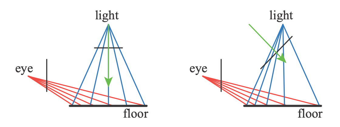
For an overhead light, on the left the sampling on the floor does not match the eye’s rate. By changing the light’s view direction and projection window on the right, the sampling rate is biased toward having a higher density of texels nearer the eye.
One lighting situation where matrix-warping techniques fail to help is when a light is in front of the camera and pointing at it. This situation is known as dueling frusta. More shadow-map samples are needed nearer the eye, but linear warping can only make the situation worse. This and other problems, such as sudden changes in quality and a “nervous,” unstable quality to the shadows produced during camera movement, have made these approaches fall out of favor.
The idea of adding more samples where the viewer is located is a good one, leading to algorithms that generate several shadow maps for a given view. The idea is simple: Generate a fixed set of shadow maps (possibly at different resolutions), covering different areas of the scene. In Blow’s scheme, four shadow maps are nested around the viewer. In this way, a high-resolution map is available for nearby objects, with the resolution dropping for those objects far away. Forsyth presents a related idea, generating different shadow maps for different visible sets of objects. The problem of how to handle the transition for objects spanning the border between two shadow maps is avoided in his setup, since each object has one and only one shadow map associated with it. Flagship Studios developed a system that blended these two ideas. One shadow map is for nearby dynamic objects, another is for a grid section of the static objects near the viewer, and a third is for the static objects in the scene as a whole. The first shadow map is generated each frame. The other two could be generated just once, since the light source and geometry are static. While all these particular systems are now quite old, the ideas of multiple maps for different objects and situations, some precomputed and some dynamic, is a common theme among algorithms that have been developed since.
Cascaded Shadow Maps
Another idea is to divide the view frustum’s volume into a few pieces by slicing it parallel to the view direction. As depth increases, each successive volume has about two to three times the depth range of the previous volume. For each view volume, the light source can make a frustum that tightly bounds it and then generate a shadow map. By using texture atlases or arrays, the different shadow maps can be treated as one large texture object, thus minimizing cache access delays. Engel’s name for this algorithm, cascaded shadow maps (CSM), is more commonly used than Zhang’s term, parallel-split shadow maps, but both appear in the literature and are effectively the same.
This type of algorithm is straightforward to implement, can cover huge scene areas with reasonable results, and is robust. The dueling frusta problem can be addressed by sampling at a higher rate closer to the eye, and there are no serious worst-case problems. Because of these strengths, cascaded shadow mapping is used in many applications.
While it is possible to use perspective warping to pack more samples into subdivided areas of a single shadow map, the norm is to use a separate shadow map for each cascade. From the viewer’s perspective, the area covered by each map can vary. Smaller view volumes for the closer shadow maps provide more samples where they are needed. Determining how the range of z-depths is split among the maps, a task called z-partitioning can be quite simple or involved. One method is logarithmic partitioning, where the ratio of far to near plane distances is made the same for each cascade map: \(r=\sqrt[c]{\frac{f}{n}}\) where $n$ and $f$ are the near and far planes of the whole scene, $c$ is the number of maps, and $r$ is the resulting ratio.
The initial near depth has a large effect on this partitioning. If the near depth was very low, this would mean that each shadow map generated must cover a larger area, lowering its precision. In practice such a partitioning gives considerable resolution to the area close to the near plane, which is wasted if there are no objects in this area. One way to avoid this mismatch is to set the partition distances as a weighted blend of logarithmic and equidistant distributions, but it would be better still if we could determine tight view bounds for the scene.
The challenge is in setting the near plane. If set too far from the eye, objects may be clipped by this plane, an extremely bad artifact. For a cut scene, an artist can set this value precisely in advance, but for an interactive environment the problem is more challenging. Lauritzen et al. present sample distribution shadow maps (SDSM), which use the z-depth values from the previous frame to determine a better partitioning by one of two methods.
The first method is to look through the z-depths for the minimum and maximum values and use these to set the near and far planes. This is performed using what is called a reduce operation on the GPU, in which a series of ever-smaller buffers are analyzed by a compute or other shader, with the output buffer fed back as input, until a 1 x 1 buffer is left. Normally, the values are pushed out a bit to adjust for the speed of movement of objects in the scene. Unless corrective action is taken, nearby objects entering from the edge of the screen may still cause problems for a frame, though will quickly be corrected in the next.
The second method also analyzes the depth buffer’s values, making a graph called a histogram that records the distribution of the z-depths along the range. In addition to finding tight near and far planes, the graph may have gaps in it where there are no objects at all. Any partition plane normally added to such an area can be snapped to where objects actually exist, giving more z-depth precision to the set of cascade maps.
In practice, the first method is general, is quick (typically in the 1 ms range per frame), and gives good results, so it has been adopted in several applications.
As with a single shadow map, shimmering artifacts due to light samples moving frame to frame are a problem, and can be even worse as objects move between cascades. A variety of methods are used to maintain stable sample points in world space, each with their own advantages. A sudden change in a shadow’s quality can occur when an object spans the boundary between two shadow maps. One solution is to have the view volumes slightly overlap. Samples taken in these overlap zones gather results from both adjoining shadow maps and are blended. Alternately, a single sample can be taken in such zone by using dithering.
Due to its popularity, considerable effort has been put into improving efficiency and quality .
- If nothing changes within a shadow map’s frustum, that shadow map does not need to be recomputed. For each light, the list of shadow casters can be precomputed by finding which objects are visible to the light, and of these, which can cast shadows on receivers .
- Since it is fairly difficult to perceive whether a shadow is correct, some shortcuts can be taken that are applicable to cascades and other algorithms. One technique is to use a low level of detail model as a proxy to actually cast the shadow . Another is to remove tiny occluders from consideration .
- The more distant shadow maps may be updated less frequently than once a frame, on the theory that such shadows are less important. This idea risks artifacts caused by large moving objects, so needs to be used with care .
- Day presents the idea of “scrolling” distant maps from frame to frame, the idea being that most of each static shadow map is reusable frame to frame, and only the fringes may change and so need rendering. Games such as DOOM (2016) maintain a large atlas of shadow maps, regenerating only those where objects have moved .
- The farther cascaded maps could be set to ignore dynamic objects entirely, since such shadows may contribute little to the scene. With some environments, a high-resolution static shadow map can be used in place of these farther cascades, which can significantly reduce the workload .
- A sparse texture system (Section 19.10.1) can be employed for worlds where a single static shadow map would be enormous .
- Cascaded shadow mapping can be combined with baked-in light-map textures or other shadow techniques that are more appropriate for particular situations .
Creating several separate shadow maps means a run through some set of geometry for each. A number of approaches to improve efficiency have been built on the idea of rendering occluders to a set of shadow maps in a single pass. The geometry shader can be used to replicate object data and send it to multiple views . Instanced geometry shaders allow an object to be output into up to 32 depth textures . Multiple-viewport extensions can perform operations such as rendering an object to a specific texture array slice . Section 21.3.1 discusses these in more detail, in the context of their use for virtual reality. A possible drawback of viewport-sharing techniques is that the occluders for all the shadow maps generated must be sent down the pipeline, versus the set found to be relevant to each shadow map .
You yourself are currently in the shadows of billions of light sources around the world. Light reaches you from only a few of these. In real-time rendering, large scenes with multiple lights can become swamped with computation if all lights are active at all times. If a volume of space is inside the view frustum but not visible to the eye, objects that occlude this receiver volume do not need to be evaluated . Bittner et al. use occlusion culling (Section 19.7) from the eye to find all visible shadow receivers, and then render all potential shadow receivers to a stencil buffer mask from the light’s point of view. This mask encodes which visible shadow receivers are seen from the light. To generate the shadow map, they render the objects from the light using occlusion culling and use the mask to cull objects where no receivers are located. Various culling strategies can also work for lights. Since irradiance falls off with the square of the distance, a common technique is to cull light sources after a certain threshold distance. For example, the portal culling technique in Section 19.5 can find which lights affect which cells. This is an active area of research, since the performance benefits can be considerable.