Particle Collision Detection and Response
Concept: Signed Distance Field (omitted)
The corresponding operation of AND bool operation is
\[inside: \phi(\mathbf{x}) = \max \{\phi_i(\mathbf{x})\}\]OR operation is
\[inside: \phi(\mathbf{x}) \approx \min \{\phi_i(\mathbf{x})\}\] \[outside: \phi(\mathbf{x}) = \min \{\phi_i(\mathbf{x})\}\]Penalty methods
Quadratic Penalty Method
When the collision is detected, a penalty method applies a penalty force in the next update. When the penalty potential is quadratic, the force is linear, which works like a spring.
Is $\phi(\mathbf{x})$ negative? Yes, then apply a force in the next update:
\[f = -k\phi(\mathbf{x})\nabla\phi(\mathbf{x})=-k\phi(\mathbf{x})\mathbf{n}\]where $k$ is the stiffness of the penalty force.
Since this method work only when penetration happens, there will always be artifacts. { : .prompt-tip }
Quadratic Penalty Method with a Buffer
A buffer helps lessen the penetration issue. But it cannot strictly prevent penetration, no matter how large k is.
Is $\phi(\mathbf{x}) < \epsilon$ ? Yes, then apply a force in the next update:
\[f =k(\epsilon - \phi(\mathbf{x}))\mathbf{n}\]When k is small, when the object is fast, the force will be too small to prevent penetration. { : .prompt-warning }
When k is large, there will be a phenomenon called over-shooting. { : .prompt-warning }
Log-Barrier Penalty Method
A log-barrier penalty method ensures that the force can be large enough when object is close, and small enough when object is far away. But it assumes $\phi(\mathbf{x}) > 0$. To achieve that, it needs to adjust $\Delta t$.
Always apply the penalty force as:
\[f = \rho\frac{1}{\phi(\mathbf{x})}\mathbf{n}\]where $\rho$ is barrier strength.
When the object is already inside, the force will pull it in even more. { : .prompt-warning }
Short Summary of Penalty Methods
- The use of step size $\Delta t$ adjustment is crucial.
- avoid over-shooting
- avoid penetration in log-barrier penalty method
- Log-barrier method can be limited within a buffer as well.
- Frictional contacts are difficult to handle.
Impulse methods
An impulse method assumes that the collision changes the position and the velocity all of sudden instead of update it in the next update.
Is $\phi(\mathbf{x}) < 0$ ? Yes, then for the new position:
\[\mathbf{x} ^{new} = \mathbf{x} - \phi(\mathbf{x})\nabla\phi(\mathbf{x})=\mathbf{x} + \vert \phi(\mathbf{x})\vert\mathbf{n}\]for the new velocity, if $\mathbf{v} \cdot \mathbf{n} < 0$, then:
\[define: \mathbf{v}_{t} = \mathbf{v} - (\mathbf{v} \cdot \mathbf{n})\mathbf{n}, \quad \mathbf{v}_{n} = (\mathbf{v} \cdot \mathbf{n})\mathbf{n}\] \[\mathbf{v_n}^{new} = -\mu_N\mathbf{v_n}, \quad \mathbf{v_t}^{new} = a\mathbf{v_t}\]where $\mu_N$ is the coefficient of restitution, with a range of (0,1).
a should be minimized but not violating Coulomb’s law:
\[\vert\vert \mathbf{v_t}^{new} - \mathbf{v_t}\vert\vert \leq \mu_T\vert\vert \mathbf{v_n}^{new} - \mathbf{v_n} \vert\vert, \quad (1-a)\vert\vert \mathbf{v_t}\vert\vert \leq \mu_T(1+\mu_N)\vert\vert \mathbf{v_n} \vert\vert\]Therefore,
\[a = \max(1-\frac{\mu_T(1+\mu_N)\vert\vert \mathbf{v_n} \vert\vert}{\vert\vert \mathbf{v_t}\vert\vert}, 0)\]where left is dynamic friction, and right is static friction.
Rigid Body Collision Detection and Response by Impulse
When encountering the rigid body collision, the velocity of the collision point $\mathbf{v}_i$ is not a state variable, which means it cannot be updated directly. Thus we need to calculate the impulse $\mathbf{j}$, and then update the velocity and angular.
Physics:
\[\mathbf{v}^{new} = \mathbf{v} - \frac{1}{m}\mathbf{j}, \quad \mathbf{\omega}^{new} = \mathbf{\omega} - \mathbf{I}^{-1}(\mathbf{R}\mathbf{r}_i\times\mathbf{j})\]where j is the impulse, and m is the mass. thus:
\[\mathbf{v}_i^{new} = \mathbf{v}_i + \frac{1}{m_i}\mathbf{j} - (\mathbf{R}\mathbf{r}_i)\times(\mathbf{I}^{-1}(\mathbf{R}\mathbf{r}_i\times\mathbf{j}))\]Cross Product as a Matrix Product
\[\mathbf{r}\times\mathbf{q} = \begin{bmatrix} 0 & -r_z & r_y \\ r_z & 0 & -r_x \\ -r_y & r_x & 0 \end{bmatrix}\begin{bmatrix} q_x \\ q_y \\ q_z \end{bmatrix} = \mathbf{r^*q}\]so that:
\[\mathbf{v}_i^{new} = \mathbf{v}_i + \frac{1}{m_i}\mathbf{j} - (\mathbf{R}\mathbf{r}_i)*(\mathbf{I}^{-1}(\mathbf{R}\mathbf{r}_i)^*\mathbf{j})\] \[\mathbf{v}_i^{new} - \mathbf{v}_i = \mathbf{Kj},\quad \mathbf{K} = \frac{1}{m}\mathbf{1} - (\mathbf{R}\mathbf{r}_i)^*\mathbf{I}^{-1}(\mathbf{R}\mathbf{r}_i)^*\]Algorithm
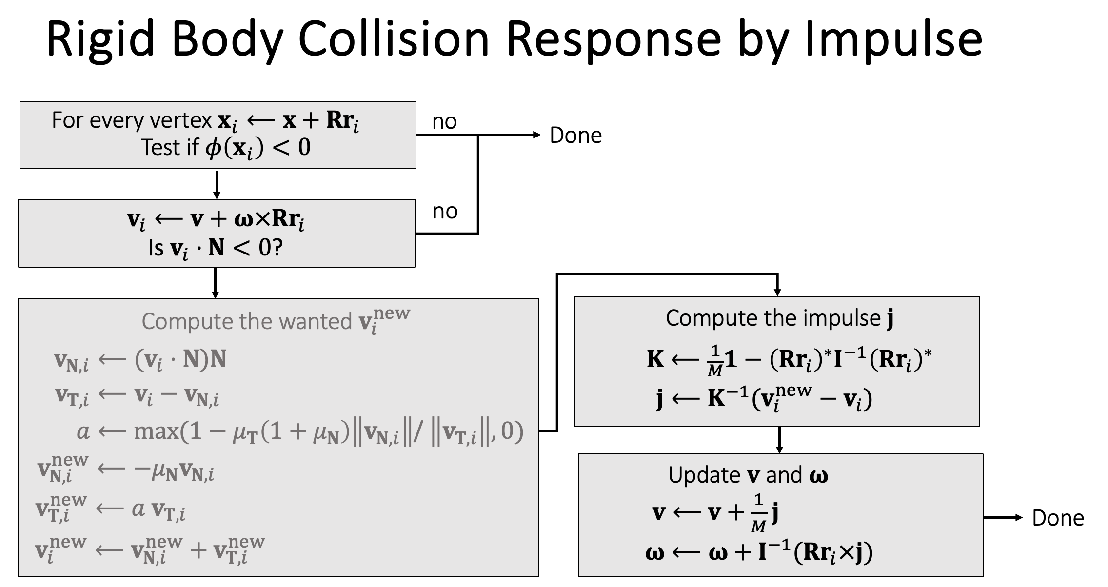
Implementation Details
- If there are many vertices in collision, we use their average position.
- We can decrease the restitution $\mu_N$ to reduce oscillation.
We don’t update the position here. Why?
- Because the problem is nonlinear.
- We will come back to this later when we talk about constraints.
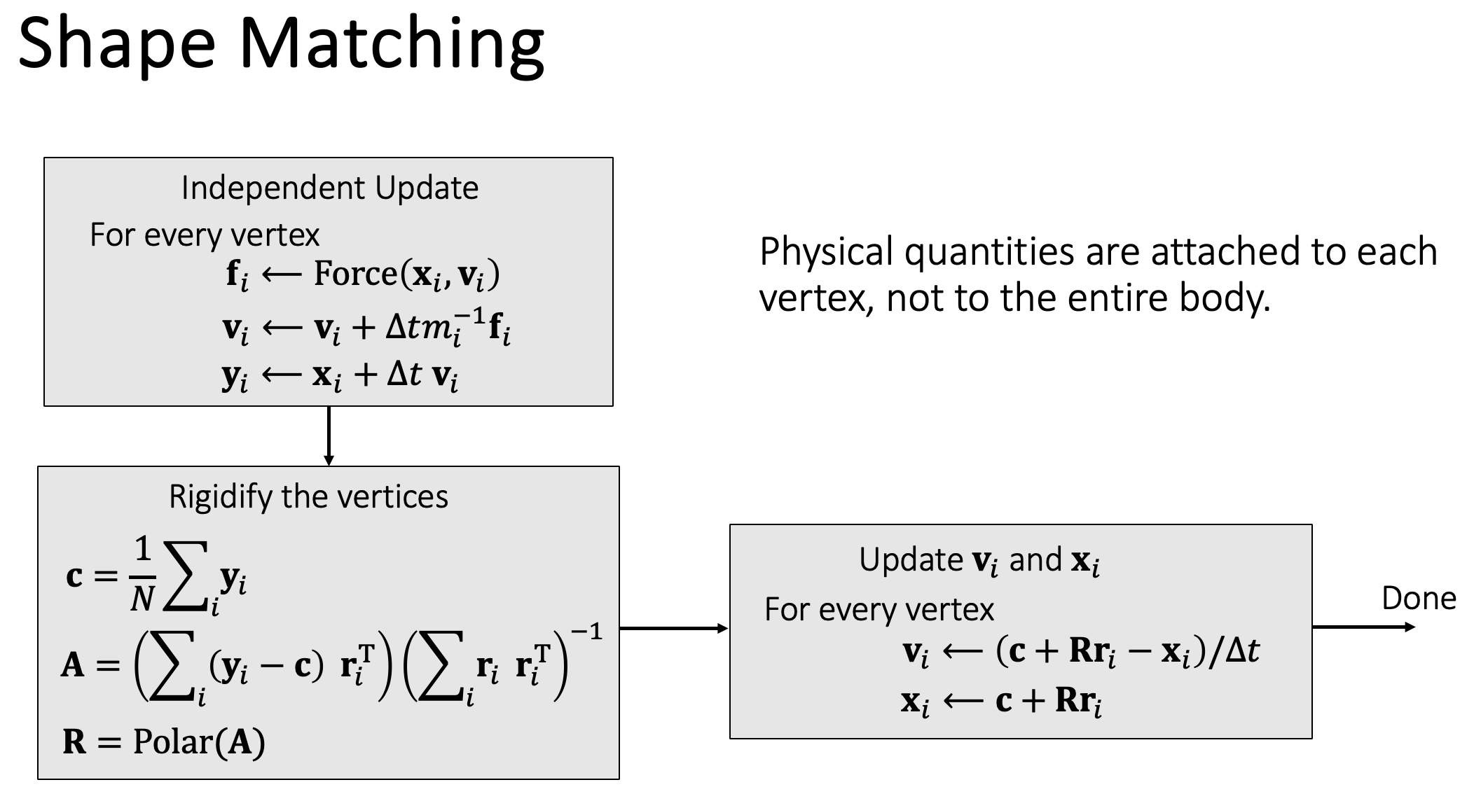
Shape Matching
Basic Idea
- We allow each vertex to have its own velocity, so it can move by itself.
- First, move vertices independently by its velocity, with collision and friction being handled.
- Second, enforce the rigidity constraint to become a rigid body again.
Mathematical Formulation
After the first step, we get new positions $\mathbf{y}_i$, and then we regulate it with:
\[\mathbf{x}_i = \mathbf{c+Rr}_i, \quad \{\mathbf{c, R}\} = \arg\min_{c, R}\sum_i\frac{1}{2}\vert\vert\mathbf{y}_i - (\mathbf{c+Rr}_i)\vert\vert^2\]where c is the center of mass, and R is the rotation matrix. Since the rotation matrix constraint brings additional complexity, we can first neglect this constraint and use the polar decomposition to achieve it. Description below:
\[\{\mathbf{c,A}\} = \arg\min_{c, A}\sum_i\frac{1}{2}\vert\vert\mathbf{y}_i - (\mathbf{c+Ar}_i)\vert\vert^2 = \arg\min_{c, A}E\]where A is ANY matrix.
solve for c and A:
\[\frac{\partial E}{\partial c} = 0, \quad \frac{\partial E}{\partial A} = 0\] \[\sum_i(\mathbf{y}_i - (\mathbf{c+Ar}_i)) = 0, \quad \sum_i(\mathbf{y}_i - (\mathbf{c+Ar}_i))\mathbf{r}_i^T = 0\]thus:
\[\mathbf{c} = \frac{1}{n}\sum_i\mathbf{y}_i, \quad \mathbf{A} = (\sum_i(\mathbf{y}_i - \mathbf{c})\mathbf{r}_i^T)(\sum_i\mathbf{r}_i\mathbf{r}_i^T)^{-1} = \mathbf{RS}\]where the last step is the polar decomposition.
Algorithm
Summary
- Easy to implement and compatible with other nodal systems, i.e., cloth, soft bodies and even particle fluids.
Difficult to strictly enforce friction and other goals.
- The rigidification process will destroy them.
- More suitable when the friction accuracy is unimportant, i.e., buttons on clothes.