Percentage-Closer Filtering
A simple extension of the shadow-map technique can provide pseudo-soft shadows. This method can also help ameliorate resolution problems that cause shadows to look blocky when a single light-sample cell covers many screen pixels. The solution is similar to texture magnification (Section 6.2.1). Instead of a single sample being taken off the shadow map, the four nearest samples are retrieved. The technique does not interpolate between the depths themselves, but rather the results of their comparisons with the surface’s depth. That is, the surface’s depth is compared separately to the four texel depths, and the point is then determined to be in light or shadow for each shadow-map sample. These results, i.e., 0 for shadow and 1 for light, are then bilinearly interpolated to calculate how much the light actually contributes to the surface location. This filtering results in an artificially soft shadow. These penumbrae change, depending on the shadow map’s resolution, camera location, and other factors. For example, a higher resolution makes for a narrower softening of the edges. Still, a little penumbra and smoothing is better than none at all.
This idea of retrieving multiple samples from a shadow map and blending the results is called percentage-closer filtering (PCF) .Area lights produce soft shadows. The amount of light reaching a location on a surface is a function of what proportion of the light’s area is visible from the location. PCF attempts to approx- imate a soft shadow for a punctual (or directional) light by reversing the process. Instead of finding the light’s visible area from a surface location, it finds the visibility of the punctual light from a set of surface locations near the original location. See Figure 7.22. The name “percentage-closer filtering” refers to the ultimate goal, to find the percentage of the samples taken that are visible to the light. This percentage is how much light then is used to shade the surface.
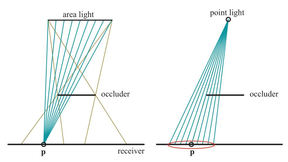
On the left, the brown lines from the area light source show where penumbrae are formed. For a single point p on the receiver, the amount of illumination received could be computed by testing a set of points on the area light’s surface and finding which are not blocked by any occluders. On the right, a point light does not cast a penumbra. PCF approximates the effect of an area light by reversing the process: At a given location, it samples over a comparable area on the shadow map to derive a percentage of how many samples are illuminated. The red ellipse shows the area sampled on the shadow map. Ideally, the width of this disk is proportional to the distance between the receiver and occluder.
In PCF, locations are generated nearby to a surface location, at about the same depth, but at different texel locations on the shadow map. Each location’s visibility is checked, and these resulting boolean values, lit or unlit, are then blended to get a soft shadow. Note that this process is non-physical: Instead of sampling the light source directly, this process relies on the idea of sampling over the surface itself. The distance to the occluder does not affect the result, so shadows have similar-sized penumbrae. Nonetheless this method provides a reasonable approximation in many situations.
Once the width of the area to be sampled is determined, it is important to sample in a way that avoids aliasing artifacts. There are numerous variations of how to sample and filter nearby shadow-map locations. Variables include how wide of an area to sample, how many samples to use, the sampling pattern, and how to weight the results. With less-capable APIs, the sampling process could be accelerated by a special texture sampling mode similar to bilinear interpolation, which accesses the four neighboring locations. Instead of blending the results, each of the four samples is compared to a given value, and the ratio that passes the test is returned . However, performing nearest neighbor sampling in a regular grid pattern can create noticeable artifacts. Using a joint bilateral filter that blurs the result but respects object edges can improve quality while avoiding shadows leaking onto other surfaces .
DirectX 10 introduced single-instruction bilinear filtering support for PCF, giving a smoother result . This offers considerable visual improvement over nearest neighbor sampling, but artifacts from regular sampling remain a problem. One solution to minimize grid patterns is to sample an area using a precomputed Poisson distribution pattern, as illustrated in Figure 7.23. This distribution spreads samples out so that they are neither near each other nor in a regular pattern. It is well known that using the same sampling locations for each pixel, regardless of the distribution, can result in patterns . Such artifacts can be avoided by randomly rotating the sample distribution around its center, which turns aliasing into noise. Castano found that the noise produced by Poisson sampling was particularly noticeable for their smooth, stylized content. He presents an efficient Gaussian-weighted sampling scheme based on bilinear sampling.
Self-shadowing problems and light leaks, i.e., acne and Peter Panning, can become worse with PCF. Slope scale bias pushes the surface away from the light based purely on its angle to the light, with the assumption that a sample is no more than a texel away on the shadow map. By sampling in a wider area from a single location on a surface, some of the test samples may get blocked by the true surface.
A few different additional bias factors have been invented and used with some success to reduce the risk of self-shadowing.Burley describes the bias cone, where each sample is moved toward the light proportional to its distance from the original sample. Burley recommends a slope of 2.0, along with a small constant bias.
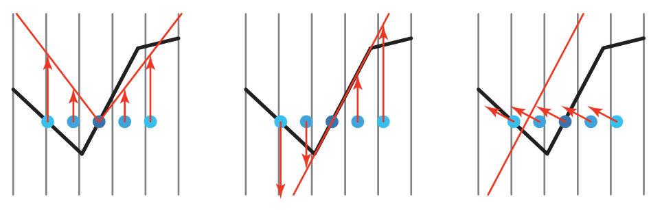
Additional shadow bias methods. For PCF, several samples are taken surrounding the original sample location, the center of the five dots. All these samples should be lit. In the left figure, a bias cone is formed and the samples are moved up to it. The cone’s steepness could be increased to pull the samples on the right close enough to be lit, at the risk of increasing light leaks from other samples elsewhere (not shown) that truly are shadowed. In the middle figure, all samples are adjusted to lie on the receiver’s plane. This works well for convex surfaces but can be counterproductive at concavities, as seen on the left side. In the right figure, normal offset bias moves the samples along the surface’s normal direction, proportional to the sine of the angle between the normal and the light. For the center sample, this can be thought of as moving to an imaginary surface above the original surface. This bias not only affects the depth but also changes the texture coordinates used to test the shadow map.
Schuler , Isidoro , and Tuft present techniques based on the ob- servation that the slope of the receiver itself should be used to adjust the depths of the rest of the samples. Of the three, Tuft’s formulation is most easily applied to cascaded shadow maps. Dou et al. further refine and extend this concept, accounting for how the z-depth varies in a nonlinear fashion. These approaches assume that nearby sample locations are on the same plane formed by the triangle. Referred to as receiver plane depth bias or other similar terms, this technique can be quite precise in many cases, as locations on this imaginary plane are indeed on the surface, or in front of it if the model is convex. Samples near concavities can become hidden. Combinations of constant, slope scale, receiver plane, view bias, and normal offset biasing have been used to combat the problem of self-shadowing, though hand-tweaking for each environment can still be necessary .
One problem with PCF is that because the sampling area’s width remains constant, shadows will appear uniformly soft, all with the same penumbra width. This may be acceptable under some circumstances, but appears incorrect where there is ground contact between the occluder and receiver.