Microfacet Theory
Many BRDF models are based on a mathematical analysis of the effects of microgeometry on reflectance called microfacet theory. This tool was first developed by researchers in the optics community . It was introduced to computer graphics in 1977 by Blinn and again in 1981 by Cook and Torrance . The theory is based on the modeling of microgeometry as a collection of microfacets.
Each of these tiny facets is flat, with a single microfacet normal $m$. The microfacets individually reflect light according to the micro-BRDF $f_\mu(l, v, m)$, with the combined reflectance across all the microfacets adding up to the overall surface BRDF. The usual choice is for each microfacet to be a perfect Fresnel mirror, resulting in a specular microfacet BRDF for modeling surface reflection. However, other choices are possible. Diffuse micro-BRDFs have been used to create several local subsurface scattering models . A diffraction micro-BRDF was used to create a shading model combining geometrical and wave optics effects .
An important property of a microfacet model is the statistical distribution of the microfacet normals $m$. This distribution is defined by the surface’s normal distribution function, or NDF. Some references use the term distribution of normals to avoid confusion with the Gaussian normal distribution. We will use \(D(m)\) to refer to the NDF in equations.
The NDF $D(m)$ is the statistical distribution of microfacet surface normals over the microgeometry surface area . Integrating $D(m)$ over the entire sphere of microfacet normals gives the area of the microsurface. More usefully, integrating $D(m)(n \cdot m)$, the projection of $D(m)$ onto the macrosurface plane, gives the area of the macrosurface patch that is equal to 1 by convention, as shown on the left side of Figure 9.31. In other words, the projection $D(m)(n \cdot m)$ is normalized:
\[\int_{m\in \Theta} D(m)(n \cdot m) dm = 1\tag{9.21}\]The integral is over the entire sphere, represented here by $\Theta$, unlike previous spherical integrals in this chapter that integrated over only the hemisphere centered on $n$, represented by $\Omega$. This notation is used in most graphics publications, though some references use $\Omega$ to denote the complete sphere. In practice, most microstructure models used in graphics are heightfields, which means that $D(m) = 0$ for all directions m outside $\Omega$. However, Equation above is valid for non-heightfield microstructures as well.
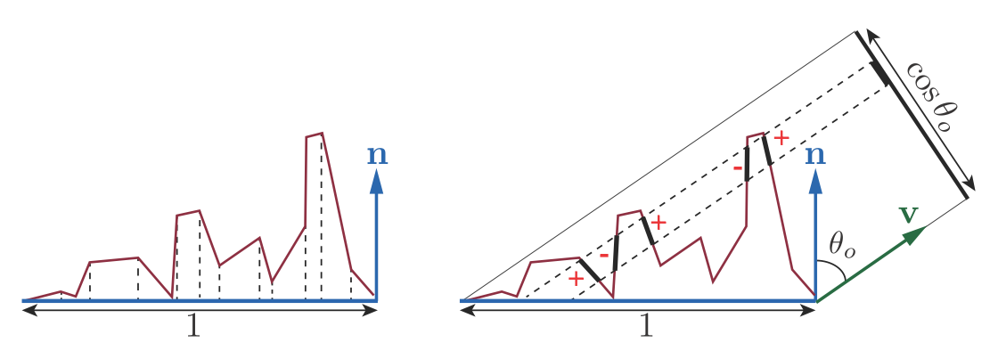
Figure 9.31. Side view of a microsurface. On the left, we see that integrating $D(m)(n \cdot m)$, the microfacet areas projected onto the macrosurface plane, yields the area (length, in this side view) of the macrosurface, which is 1 by convention. On the right, integrating $D(m)(v \cdot m)$, the microfacet areas projected onto the plane perpendicular to $v$, yields the projection of the macrosurface onto that plane, which is cos $\theta_o$ or $(v \cdot n)$. When the projections of multiple microfacets overlap, the negative projected areas of the backfacing microfacets cancel out the “extra” frontfacing microfacets.
More generally, the projections of the microsurface and macrosurface onto the plane perpendicular to any view direction $v$ are equal:
\[\int_{m\in \Theta} D(m)(v \cdot m) dm = v \cdot n \tag{9.22}\]The dot products in the two Equations above are not clamped to 0. The right side of Figure 9.31 shows why. Equations impose constraints that the function $D(m)$ must obey to be a valid NDF.
Intuitively, the NDF is like a histogram of the microfacet normals. It has high values in directions where the microfacet normals are more likely to be pointing. Most surfaces have NDFs that show a strong peak at the macroscopic surface normal $n$. Section 9.8.1 will cover several NDF models used in rendering.
Take a second look at the right side of Figure 9.31. Although there are many microfacets with overlapping projections, ultimately for rendering we care about only the visible microfacets, i.e., the microfacets that are closest to the camera in each overlapping set. This fact suggests an alternative way of relating the projected microfacet areas to the projected macrogeometry area: The sum of the projected areas of the visible microfacets is equal to the projected area of the macrosurface. We can express this mathematically by defining the masking function $G_1(m, v)$, which gives the fraction of microfacets with normal $m$ that are visible along the view vector $v$. The integral of $G_1(m, v)D(m)(v \cdot m)^+$ over the sphere then gives the area of the macrosurface projected onto the plane perpendicular to $v$:
\[\int_{m\in \Theta} G_1(m, v)D(m)(v \cdot m)^+ dm = v \cdot n\tag{9.23}\]as shown in Figure 9.32. The dot product in Equation above is clamped to zero. Backfacing microfacets are not visible, so they are not counted in this case. The product $G_1(m, v)D(m)$ is the distribution of visible normals .
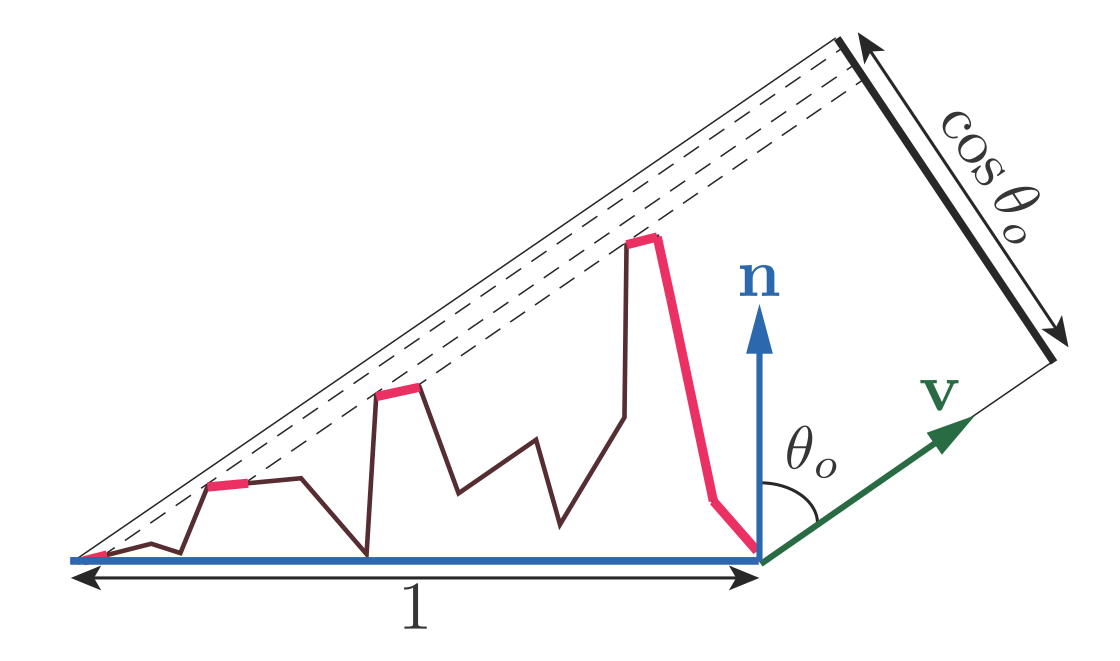
Figure 9.32. Integrating the projected areas of the visible microfacets (in bright red) yields the projected area of the macrosurface onto the plane perpendicular to $v$.
While Equation above imposes a constraint on $G_1(m, v)$, it does not uniquely determine it. There are infinite functions that satisfy the constraint for a given microfacet normal distribution $D(m)$ . This is because $D(m)$ does not fully specify the microsurface. It tells us how many of the microfacets have normals pointing in certain directions, but not how they are arranged.
Although various $G_1$ functions have been proposed over the years, the dilemma as to which one to use has been solved (at least for now) in an excellent paper by Heitz . Heitz discusses the Smith masking function, which was initially derived for Gaussian normal distributions and later generalized to arbitrary NDFs . Heitz shows that out of the masking functions proposed in the literature, only two?the Smith function and the Torrance-Sparrow “V-cavity” function ?obey Equation above and are thus mathematically valid. He further shows that the Smith function is a much closer match to the behavior of random microsurfaces than the TorranceSparrow function. Heitz also proves that the Smith masking function is the only possible function that both obeys Equation above and possesses the convenient property of normal-masking independence. This means that the value of $G_1(m, v)$ does not depend on the direction of $m$ as long as $m$ is not backfacing i.e., as long as $m \cdot v \leq 0$. The Smith $G_1$ function has the following form:
\[G_1(m, v) = \frac{\chi^+(m \cdot v)}{1 + \Lambda(v)} \tag{9.24}\]where $\chi^+$ is the positive characteristic function \(\chi^+(x) = 1, where x > 0; 0, where x \leq 0\tag{9.25}\). The $\Lambda$ function differs for each NDF. The procedure to derive $\Lambda$ for a given NDF is described in publications by Walter et al. and Heitz .
The Smith masking function does have some drawbacks. From a theoretical standpoint, its requirements are not consistent with the structure of actual surfaces , and may even be physically impossible to realize . From a practical standpoint, while it is quite accurate for random surfaces, its accuracy is expected to decrease for surfaces with a stronger dependency between normal direction and masking, such as the surface shown in Figure 9.28, especially if the surface has some repetitive structure (as do most fabrics). Nevertheless, until a better alternative is found, it is the best option for most rendering applications.
Given a microgeometry description including a micro-BRDF $f_\mu(l, v, m)$, normal distribution function $D(m)$, and masking function $G_1(m, v)$, the overall macrosurface BRDF can be derived:
\[f(l,v)=\int_{m\in\Omega}f_\mu(l,v,m)G_2(l,v,m)D(m)\frac{(m\cdot l)^+}{\vert n\cdot l \vert}\frac{(m\cdot v)^+}{\vert n \cdot v \vert}dm \tag{9.26}\]This integral is over the hemisphere $\Omega$ centered on $n$, to avoid collecting light contributions from under the surface. Instead of the masking function $G_1(m, v)$, Equation above uses the joint masking-shadowing function $G_2(l, v, m)$. This function, derived from $G_1$, gives the fraction of microfacets with normal $m$ that are visible from two directions: the view vector $v$ and the light vector $l$. By including the $G_2$ function, Equation 9.26 enables the BRDF to account for masking as well as shadowing, but not for interreflection between microfacets (see Figure 9.27). The lack of microfacet interreflection is a limitation shared by all BRDFs derived from Equation 9.26. Such BRDFs are somewhat too dark as a result. In Sections 9.8.2 and 9.9, we will discuss some methods that have been proposed to address this limitation.
Heitz discusses several versions of the $G_2$ function. The simplest is the separable form, where masking and shadowing are evaluated separately using $G_1$ and multiplied together:
\[G_2(l, v, m) = G_1(m, l)G_1(m, v) \tag{9.27}\]This form is equivalent to assuming that masking and shadowing are uncorrelated events. In reality they are not, and the assumption causes over-darkening in BRDFs using this form of $G_2$.
As an extreme example, consider the case when the view and light directions are the same. In this case $G_2$ should be equal to $G_1$, since none of the visible facets are shadowed, but with Equation 9.27 $G_2$ will be equal to $G_1^2$ instead.
If the microsurface is a heightfield, which is typically the case for microsurface models used in rendering, then whenever the relative azimuth angle $\psi$ between $v$ and $l$ is equal to $0^\circ$, $G_2(l, v, m)$ should be equal to $\min(G_1(v, m), G_1(l, m))$. See Figure 9.17 on for an illustration of $\psi$. This relationship suggests a general way to account for correlation between masking and shadowing that can be used with any $G_1$ function:
\[G_2(l, v, m) = \lambda(\phi)G_1(v, m)G_1(l, m) + (1 - \lambda(\phi))\min(G_1(v, m), G_1(l, m)) \tag{9.28}\]where $\lambda(\psi)$ is some function that increases from 0 to 1 as the angle $\psi$ increases. Ashikhmin et al. suggested a Gaussian with a standard deviation of $15^\circ$( 0.26 radians):
\[\lambda(\psi)=1-e^{-7.3\psi^2} \tag{9.29}\]A different $\lambda$ function was proposed by van Ginneken et al.:
\[\lambda(\psi)=\frac{4.41\psi}{4.41\psi+1} \tag{9.30}\]Regardless of the relative alignment of the light and view directions, there is another reason that masking and shadowing at a given surface point are correlated. Both are related to the point’s height relative to the rest of the surface. The probability of masking increases for lower points, and so does the probability of shadowing. If the Smith masking function is used, this correlation can be precisely accounted for by the Smith height-correlated masking-shadowing function:
\[G_2(l,v,m)=\frac{\chi^+(m \cdot v)\chi^+(m \cdot l)}{1+\Lambda(v)+\Lambda(l)} \tag{9.31}\]Heitz also describes a form of Smith $G_2$ that combines direction and height correlation:
\[G_2(l,v,m)=\frac{\chi^+(m \cdot v)\chi^+(m \cdot l)}{1+\max(\Lambda(v),\Lambda(l))+\lambda(v,l)\min(\Lambda(v),\Lambda(l))} \tag{9.32}\]where the function $\lambda(v, l)$ could be an empirical function such as the ones in Equations 9.29 and 9.30, or one derived specifically for a given NDF.
Out of these alternatives, Heitz recommends the height-correlated form of the Smith function (Equation 9.31) since it has a similar cost to the uncorrelated form and better accuracy. This form is the most widely used in practice , though some practitioners use the separable form (Equation 9.27) .
The general microfacet BRDF (Equation 9.26) is not used directly for rendering. It is used to derive a closed-form solution (exact or approximate) given a specific choice of micro-BRDF $f_\mu$. The first example of this type of derivation will be shown in the next section.