Many of the RGB color values discussed in previous chapters represent intensities and shades of light. In this chapter we will learn about the various physical light quantities measured by these values, laying the groundwork for subsequent chapters, which discuss rendering from a more physically based perspective. We will also learn more about the often-neglected “second half” of the rendering process: the transformation of colors that represent scene linear light quantities into final display colors.
Light Quantities
The first step in any physically based approach to rendering is to quantify light in a precise manner. Radiometry is presented first, as this is the core field concerned with the physical transmission of light. We follow with a discussion of photometry, which deals with light values that are weighted by the sensitivity of the human eye. Our perception of color is a psychophysical phenomenon: the psychological perception of physical stimuli. Color perception is discussed in the section on colorimetry. Finally, we discuss the validity of rendering with RGB color values.
Radiometry
Radiometry deals with the measurement of electromagnetic radiation. As will be discussed in more detail in Section 9.1, this radiation propagates as waves.
Radiometric quantities exist for measuring various aspects of electromagnetic radiation: overall energy, power (energy over time), and power density with respect to area, direction, or both. These quantities are summarized below.
| Name | Symbol | Units |
|---|---|---|
| radiant flux | $\Phi$ | W (watts) |
| irradiance | $E$ | W/m |
| radiant intensity | $I$ | W/sr (watts per steradian) |
| radiance | $L$ | W/(m * sr) |
In radiometry, the basic unit is radiant flux, $\Phi$. Radiant flux is the flow of radiant energy over time?power?measured in watts (W).
Irradiance is the density of radiant flux with respect to area, i.e., $d\Phi/dA$. Irradiance is defined with respect to an area, which may be an imaginary area in space, but is most often the surface of an object. It is measured in watts per square meter.
Before we get to the next quantity, we need to first introduce the concept of a solid angle, which is a three-dimensional extension of the concept of an angle. An angle can be thought of as a measure of the size of a continuous set of directions in a plane, with a value in radians equal to the length of the arc this set of directions intersects on an enclosing circle with radius 1. Similarly, a solid angle measures the size of a continuous set of directions in three-dimensional space, measured in steradians (abbreviated “sr”), which are defined by the area of the intersection patch on an enclosing sphere with radius 1 . Solid angle is represented by the symbol $\omega$. In two dimensions, an angle of $2\pi$ radians covers the whole unit circle. Extending this to three dimensions, a solid angle of $4\pi$ steradians would cover the whole area of the unit sphere.
Now we can introduce radiant intensity, I, which is flux density with respect to direction?more precisely, solid angle ($\frac{d\Phi}{d\omega}$). It is measured in watts per steradian.
Finally, radiance, $L$, is a measure of electromagnetic radiation in a single ray. More precisely, it is defined as the density of radiant flux with respect to both area and solid angle ($d^2\Phi/dAd\omega$). This area is measured in a plane perpendicular to the ray. If radiance is applied to a surface at some other orientation, then a cosine correction factor must be used. You may encounter definitions of radiance using the term “projected area” in reference to this correction factor.
Radiance is what sensors, such as eyes or cameras, measure (see Section 9.2 for more details), so it is of prime importance for rendering. The purpose of evaluating a shading equation is to compute the radiance along a given ray, from the shaded surface point to the camera. The value of $L$ along that ray is the physically based equivalent of the quantity $c_{shaded}$ in Chapter 5. The metric units of radiance are watts per square meter per steradian.
The radiance in an environment can be thought of as a function of five variables (or six, including wavelength), called the radiance distribution . Three of the variables specify a location, the other two a direction. This function describes all light traveling anywhere in space. One way to think of the rendering process is that the eye and screen define a point and a set of directions (e.g., a ray going through each pixel), and this function is evaluated at the eye for each direction. Image-based rendering, discussed in Section 13.4, uses a related concept, called the light field.
In shading equations, radiance often appears in the form $L_o(x, \vec{d})$ or $L_i(x, \vec{d})$, which mean radiance going out from the point $x$ or entering into it, respectively.
The direction vector $\vec{d}$ indicates the ray’s direction, which by convention always points away from $x$. While this convention may be somewhat confusing in the case of $L_i$, since $d$ points in the opposite direction to the light propagation, it is convenient for calculations such as dot products.
An important property of radiance is that it is not affected by distance, ignoring atmospheric effects such as fog. In other words, a surface will have the same radiance regardless of its distance from the viewer. The surface covers fewer pixels when more distant, but the radiance from the surface at each pixel is constant.
Most light waves contain a mixture of many different wavelengths. This is typically visualized as a spectral power distribution (SPD), which is a plot showing how the light’s energy is distributed across different wavelengths. Clearly, human eyes make for poor spectrometers. We will discuss color vision in detail in Section 8.1.3. All radiometric quantities have spectral distributions. Since these distributions are densities over wavelength, their units are those of the original quantity divided by nanometers. For example, the spectral distribution of irradiance has units of watts per square meter per nanometer.
Since full SPDs are unwieldy to use for rendering, especially at interactive rates, in practice radiometric quantities are represented as RGB triples. In Section 8.1.3 we will explain how these triples relate to spectral distributions.
Photometry
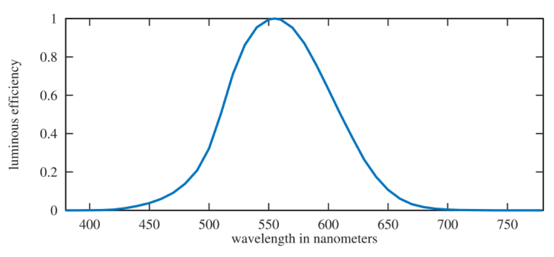
Radiometry deals purely with physical quantities, without taking account of human perception. A related field, photometry, is like radiometry, except that it weights everything by the sensitivity of the human eye. The results of radiometric computations are converted to photometric units by multiplying by the CIE photometric curve, a bell-shaped curve centered around 555 nm that represents the eye’s response to various wavelengths of light.
The full and more accurate name is the “CIE photopic spectral luminous efficiency curve.” The word “photopic” refers to lighting conditions brighter than 3.4 candelas per square meter?twilight or brighter. Under these conditions the eye’s cone cells are active. There is a corresponding “scotopic” CIE curve, centered around 507 nm, that is for when the eye has become dark-adapted to below 0.034 candelas per square meter, i.e. a moonless night or darker. The rod cells are active under these conditions.
The conversion curve and the units of measurement are the only difference between the theory of photometry and the theory of radiometry. Each radiometric quantity has an equivalent metric photometric quantity. The Table below shows the names and units of each. The units all have the expected relationships (e.g., lux is lumens per square meter). Although logically the lumen should be the basic unit, historically the candela was defined as a basic unit and the other units were derived from it. In North America, lighting designers measure illuminance using the deprecated Imperial unit of measurement, called the foot-candle (fc), instead of lux. In either case, illuminance is what most light meters measure, and it is important in illumination engineering.
| Radiometric Quantity: Units | Photometric Quantity: Units |
|---|---|
| radiant flux : W | luminous flux : lumen (lm) |
| irradiance : $W/m^2$ | illuminance : lux (lx) |
| radiant intensity : $W/sr$ | luminous intensity : candela (cd) |
| radiance : $W/m^2/sr$ | luminance : candela per square meter (cd/m2= nit) |
Luminance is often used to describe the brightness of flat surfaces. For example, high dynamic range (HDR) television screens’ peak brightness typically ranges from about 500 to 1000 nits. In comparison, clear sky has a luminance of about 8000 nits, a 60-watt bulb about 120,000 nits, and the sun at the horizon 600,000 nits.
Colorimetry
In Section 8.1.1 we have seen that our perception of the color of light is strongly connected to the light’s SPD (spectral power distribution). We also saw that this is not a simple one-to-one correspondence. Colorimetry deals with the relationship between spectral power distributions and the perception of color.
Humans can distinguish about 10 million different colors. For color perception, the eye works by having three different types of cone receptors in the retina, with each type of receptor responding differently to various wavelengths. Other animals have varying numbers of color receptors, in some cases as many as fifteen . So, for a given SPD, our brain receives only three different signals from these receptors. This is why just three numbers can be used to precisely represent any color stimulus .
But what three numbers? A set of standard conditions for measuring color was proposed by the CIE (Commission Internationale d’Eclairage), and color-matching experiments were performed using them. In color matching, three colored lights are projected on a white screen so that their colors add together and form a patch. A test color to match is projected next to this patch. The test color patch is of a single wavelength. The observer can then change the three colored lights using knobs calibrated to a range weighted [?1, 1] until the test color is matched. A negative weight is needed to match some test colors, and such a weight means that the corresponding light is added instead to the wavelength’s test color patch. One set of test results for three lights, called r, g, and b, is shown in Figure 8.5. The lights were almost monochromatic, with the energy distribution of each narrowly clustered around one of the following wavelengths: 645 nm for r, 526 nm for g, and 444 nm for b. The functions relating each set of matching weights to the test patch wavelengths are called color-matching functions.
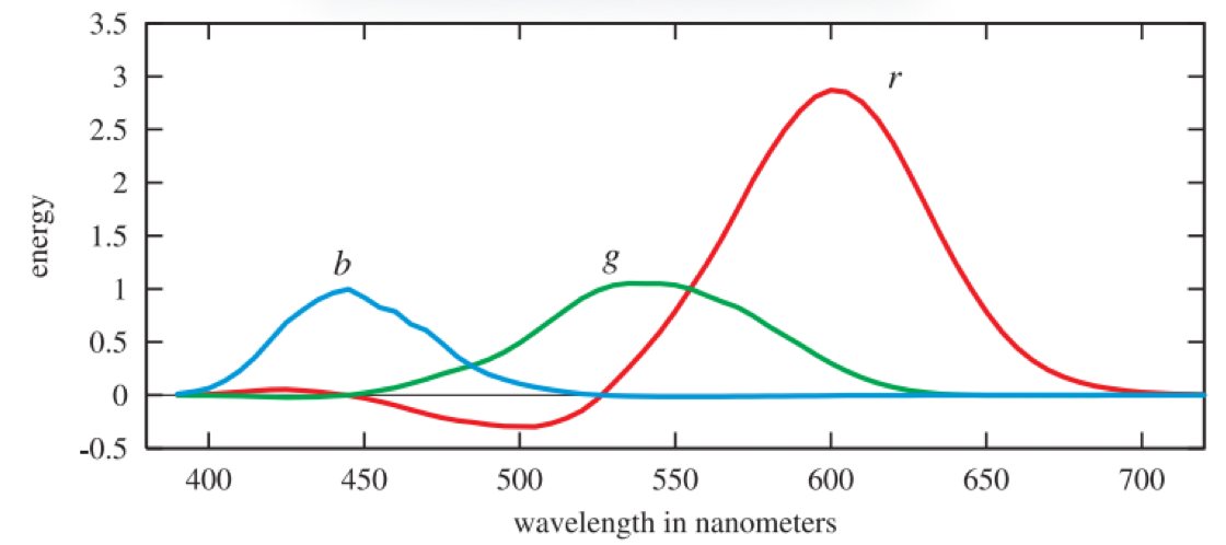
The r, g, and b 2-degree color-matching curves, from Stiles and Burch . These color-matching curves are not to be confused with the spectral distributions of the light sources used in the color-matching experiment, which are pure wavelengths.
What these functions give is a way to convert a spectral power distribution to three values. Given a single wavelength of light, the three colored light settings can be read off the graph, the knobs set, and lighting conditions created that will give an identical sensation from both patches of light on the screen. For an arbitrary spectral distribution, the color-matching functions can be multiplied by the distribution and the area under each resulting curve (i.e., the integral) gives the relative amounts to set the colored lights to match the perceived color produced by the spectrum. Considerably different spectral distributions can resolve to the same three weights, i.e., they look the same to an observer. Spectral distributions that give matching weights are called metamers.
The three weighted r, g, and b lights cannot directly represent all visible colors, as their color-matching functions have negative weights for various wavelengths. The CIE proposed three different hypothetical light sources with color-matching functions that are positive for all visible wavelengths. These curves are linear combinations of the original r, g, and b color-matching functions. This requires their spectral power distributions of the light sources to be negative at some wavelengths, so these lights are unrealizable mathematical abstractions. Their color-matching functions are denoted $\overline{x}(\lambda)$, $\overline{y}(\lambda)$, and $\overline{z}(\lambda)$, and are shown in Figure 8.6. The color-matching function $\overline{y}(\lambda)$ is the same as the photometric curve (Figure 8.4), as radiance is converted to luminance with this curve.
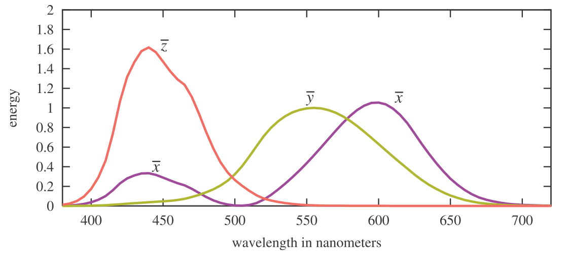
The Judd-Vos-modified CIE (1978) 2-degree color-matching functions. Note that the two x’s are part of the same curve.
As with the previous set of color-matching functions, $\overline{x}(\lambda)$, $\overline{y}(\lambda)$, and $\overline{z}(\lambda)$ are used to reduce any SPD $s(\lambda)$ to three numbers via multiplication and integration:
\[X = \int_{380}^{780}s(\lambda)\overline{x}(\lambda)d\lambda\]These X, Y , and Z tristimulus values are weights that define a color in CIE XYZ space.
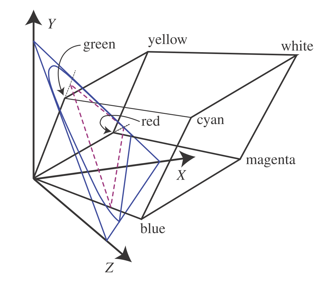
The RGB color cube for the CIE RGB primaries is shown in XYZ space, along with its projection (in violet) onto the X + Y + Z = 1 plane. The blue outline encloses the space of possible chromaticity values. Each line radiating from the origin has a constant chromaticity value, varying only in luminance.
It is often convenient to separate colors into luminance (brightness) and chromaticity. Chromaticity is the character of a color independent of its brightness. For example, two shades of blue, one dark and one light, can have the same chromaticity despite differing in luminance.
For this purpose, the CIE defined a two-dimensional chromaticity space by projecting colors onto the $X + Y + Z = 1$ plane. See Figure 8.7. Coordinates in this space are called $x$ and $y$, and are computed as follows:
\[x = \frac{X}{X + Y + Z}\] \[y = \frac{Y}{X + Y + Z}\] \[z = \frac{Z}{X + Y + Z} = 1 - x - y\]The $z$ value gives no additional information, so it is normally omitted. The plot of the chromaticity coordinates $x$ and $y$ values is known as the CIE 1931 chromaticity diagram. See Figure 8.8. The curved outline in the diagram shows where the colors of the visible spectrum lie, and the straight line connecting the ends of the spectrum is called the purple line. The black dot shows the chromaticity of illuminant D65, which is a frequently used white point–a chromaticity used to define the white or achromatic (colorless) stimulus.
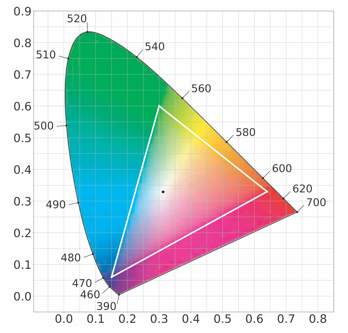
The CIE 1931 chromaticity diagram. The curve is labeled with the wavelengths of the corresponding pure colors. The white triangle and black dot show the gamut and white point, respectively, used for the sRGB and Rec. 709 color spaces.
To summarize, we began with an experiment that used three single-wavelength lights and measured how much of each was needed to match the appearance of some other wavelength of light. Sometimes these pure lights had to be added to the sample being viewed in order to match. This gave one set of color-matching functions, which were combined to create a new set without negative values. With this non-negative set of color-matching functions in hand, we can convert any spectral distribution to an XYZ coordinate that defines a color’s chromaticity and luminance, which can be reduced to $xy$ to describe just the chromaticity, keeping luminance constant.
Given a color point $(x, y)$, draw a line from the white point through this point to the boundary (spectral or purple line). The relative distance of the color point compared to the distance to the edge of the region is the excitation purity of the color. The point on the region edge defines the dominant wavelength. These colorimetric terms are rarely encountered in graphics. Instead, we use saturation and hue, which correlate loosely with excitation purity and dominant wavelength, respectively. More precise definitions of saturation and hue can be found in books by Stone and others .
The chromaticity diagram describes a plane. The third dimension needed to fully describe a color is the $Y$ value, luminance. These then define what is called the $xyY$-coordinate system. The chromaticity diagram is important in understanding how color is used in rendering, and the limits of the rendering system. A television or computer monitor presents colors by using some settings of R, G, and B color values. Each color channel controls a display primary that emits light with a particular spectral power distribution. Each of the three primaries is scaled by its respective color value, and these are added together to create a single spectral power distribution that the viewer perceives.
The triangle in the chromaticity diagram represents the gamut of a typical television or computer monitor. The three corners of the triangle are the primaries, which are the most saturated red, green, and blue colors the screen can display. An important property of the chromaticity diagram is that these limiting colors can be joined by straight lines to show the limits of the display system as a whole. The straight lines represent the limits of colors that can be displayed by mixing these three primaries. The white point represents the chromaticity that is produced by the display system when the R, G, and B color values are equal to each other. It is important to note that the full gamut of a display system is a three-dimensional volume. The chromaticity diagram shows only the projection of this volume onto a two-dimensional plane.
There are several RGB spaces of interest in rendering, each defined by R, G, and B primaries and a white point. To compare them we will use a different type of chromaticity diagram, called the CIE 1976 UCS (uniform chromaticity scale) diagram. This diagram is part of the CIELUV color space, which was adopted by the CIE (along with another color space, CIELAB) with the intention of providing more perceptually uniform alternatives to the XYZ space . Color pairs that are perceptibly different by the same amount can be up to 20 times different in distance in CIE XYZ space. CIELUV improves upon this, bringing the ratio down to a maximum of four times. This increased perceptual uniformity makes the 1976 diagram much better than the 1931 one for the purpose of comparing the gamuts of RGB spaces. Continued research into perceptually uniform color spaces has recently resulted in the $IC_TC_P$ and $J_za_zb_z$ spaces. These color spaces are more perceptually uniform than CIELUV, especially for the high luminance and saturated colors typical of modern displays. However, chromaticity diagrams based on these color spaces have not yet been widely adopted, so we use the CIE 1976 UCS diagrams in this chapter, for example in the case of Figure 8.9.
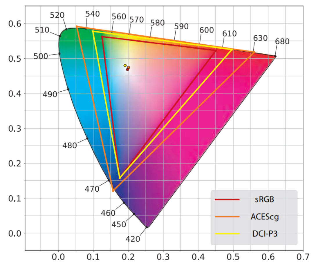
A CIE 1976 UCS diagram showing the primaries and white points of three RGB color spaces: sRGB, DCI-P3, and ACEScg. The sRGB plot can be used for Rec. 709 as well, since the two color spaces have the same primaries and white point.
Of the three RGB spaces shown in Figure 8.9, sRGB is by far the most commonly used in real-time rendering. It is important to note that in this section we use “sRGB color space” to refer to a linear color space that has the sRGB primaries and white point, and not to the nonlinear sRGB color encoding that was discussed in Section 5.6. Most computer monitors are designed for the sRGB color space, and the same primaries and white point apply to the Rec. 709 color space as well, which is used for HDTV displays and thus is important for game consoles. However, more displays are being made with wider gamuts. Some computer monitors intended for photo editing use the Adobe 1998 color space (not shown). The DCI-P3 color space?initially developed for feature film production?is seeing broader use. Apple has adopted this color space across their product line from iPhones to Macs, and other manufacturers have been following suit. Although ultra-high definition (UHD) content and displays are specified to use the extremely-wide-gamut Rec. 2020 color space, in many cases DCI-P3 is used as a de facto color space for UHD as well. Rec. 2020 is not shown in Figure 8.9, but its gamut is quite close to that of the third color space in the figure, ACEScg. The ACEScg color space was developed by the Academy of Motion Picture Arts and Sciences (AMPAS) for feature film computer graphics rendering. It is not intended for use as a display color space, but rather as a working color space for rendering, with colors converted to the appropriate display color space after rendering.
While currently the sRGB color space is ubiquitous in real-time rendering, the use of wider color spaces is likely to increase. The most immediate benefit is for applications targeting wide-gamut displays , but there are advantages even for applications targeting sRGB or Rec. 709 displays. Routine rendering operations such as multiplication give different results when performed in different color spaces , and there is evidence that performing these operations in the DCI-P3 or ACEScg space produces more accurate results than performing them in linear sRGB space .
Conversion from an RGB space to XYZ space is linear and can be done with a matrix derived from the RGB space’s primaries and white point . Via matrix inversion and concatenation, matrices can be derived to convert from XYZ to any RGB space, or between two different RGB spaces. Note that after such a conversion the RGB values may be negative or greater than one. These are colors that are out of gamut, i.e., not reproducible in the target RGB space. Various methods can be used to map such colors into the target RGB gamut .
One often-used conversion is to transform an RGB color to a grayscale luminance value. Since luminance is the same as the Y coefficient, this operation is just the “Y part” of the RGB-to-XYZ conversion. In other words, it is a dot product between the RGB coefficients and the middle row of the RGB-to-XYZ matrix. In the case of the sRGB and Rec. 709 spaces, the equation is
\[Y=0.2126R+0.7152G+0.0722B\]This brings us again to the photometric curve. This curve, representing how a standard observer’s eye responds to light of various wavelengths, is multiplied by the spectral power distributions of the three primaries, and each resulting curve is integrated. The three resulting weights are what form the luminance equation above. The reason that a grayscale intensity value is not equal parts red, green, and blue is because the eye has a different sensitivity to various wavelengths of light.
Colorimetry can tell us whether two color stimuli match, but it cannot predict their appearance. The appearance of a given XYZ color stimulus depends heavily on factors such as the lighting, surrounding colors, and previous conditions. Color appearance models (CAM) such as CIECAM02 attempt to deal with these issues and predict the final color appearance.
Color appearance modeling is part of the wider field of visual perception, which includes effects such as masking . This is where a high-frequency, high-contrast pattern laid on an object tends to hide flaws. In other words, a texture such as a Persian rug will help disguise color banding and other shading artifacts, meaning that less rendering effort needs to be expended for such surfaces.
Rendering with RGB Colors
Strictly speaking, RGB values represent perceptual rather than physical quantities. Using them for physically based rendering is technically a category error. The correct method would be to perform all rendering computations on spectral quantities, represented either via dense sampling or projection onto a suitable basis, and to convert to RGB colors only at the end.
For example, one of the most common rendering operations is calculating the light reflected from an object. The object’s surface typically will reflect light of some wavelengths more than others, as described by its spectral reflectance curve. The strictly correct way to compute the color of the reflected light is to multiply the SPD of the incident light by the spectral reflectance at each wavelength, yielding the SPD of the reflected light that would then be converted to an RGB color. Instead, in an RGB renderer the RGB colors of the lights and surface are multiplied together to give the RGB color of the reflected light. In the general case, this does not give the correct result. To illustrate, we will look at a somewhat extreme example, shown in Figure 8.10.
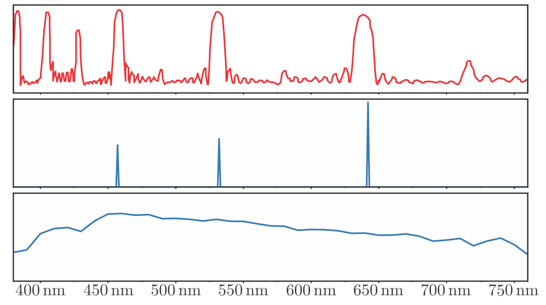
The top plot shows the spectral reflectance of a material designed for use in projection screens. The lower two plots show the spectral power distributions of two illuminants with the same RGB colors: an RGB laser projector in the middle plot and the D65 standard illuminant in the bottom plot. The screen material would reflect about 80% of the light from the laser projector because it has reflectance peaks that line up with the projectors primaries. However, it will reflect less than 20% of the light from the D65 illuminant since most of the illuminant’s energy is outside the screen’s reflectance peaks. An RGB rendering of this scene would predict that the screen would reflect the same intensity for both lights.
Our example shows a screen material designed for use with laser projectors. It has high reflectance in narrow bands matching laser projector wavelengths and low reflectance for most other wavelengths. This causes it to reflect most of the light from the projector, but absorb most of the light from other light sources. An RGB renderer will produce gross errors in this case.
However, the situation shown in Figure 8.10 is far from typical. The spectral reflectance curves for surfaces encountered in practice are much smoother. Typical illuminant SPDs resemble the D65 illuminant rather than the laser projector in the example. When both the illuminant SPD and surface spectral reflectance are smooth, the errors introduced by RGB rendering are relatively subtle.
In predictive rendering applications, these subtle errors can be important. For example, two spectral reflectance curves may have the same color appearance under one light source, but not another. This problem, called metameric failure or illuminant metamerism, is of serious concern when painting repaired car body parts, for example. RGB rendering would not be appropriate in an application that attempts to predict this type of effect.
However, for the majority of rendering systems, especially those for interactive applications, that are not aimed at producing predictive simulations, RGB rendering works surprisingly well . Even feature-film offline rendering has only recently started to employ spectral rendering, and it is as yet far from common .
This section has touched on just the basics of color science, primarily to bring an awareness of the relation of spectra to color triplets and to discuss the limitations of devices. A related topic, the transformation of rendered scene colors to display values, will be discussed in the next section.