Image Texturing | Real-time Rendering Chapter 6.2

Image Texturing

What the floating point coordinates of the center of a pixel are?

DirectX 10 onward changes to OpenGL’s system, where the center of a texel has the fractional values (0.5,0.5)—truncation, or more accurately, flooring, where the fraction is dropped. Flooring is a more natural system that maps well to language, in that pixel (5,9), for example, defines a range from 5.0 to 6.0 for the u-coordinate and 9.0 to 10.0 for the v.

One term worth explaining at this point is dependent texture read, which has two definitions.

• The first applies to mobile devices in particular. When accessing a texture via texture2D or similar, a dependent texture read occurs whenever the pixel shader calculates texture coordinates instead of using the unmodified texture coordinates passed in from the vertex shader.

• Older mobile GPUs, those that do not support OpenGL ES 3.0, run more efficiently when the shader has no dependent texture reads, as the texel data can then be prefetched.

The texture image size used in GPUs is usually 2^m × 2^n texels, where m and n are non-negative integers. These are referred to as power-of-two (POT) textures. Modern GPUs can handle non-power-of-two (NPOT) textures of arbitrary size, which allows a generated image to be treated as a texture. However, some older mobile GPUs may not support mipmapping for NPOT textures. Graphics accelerators have different upper limits on texture size.

The image sampling and filtering methods discussed in this chapter are applied to the values read from each texture.

However, the desired result is to prevent aliasing in the final rendered image, which in theory requires sampling and filtering the final pixel colors. The distinction here is between filtering the inputs to the shading equation, or filtering its output. As long as the inputs and output are linearly related (which is true for inputs such as colors), then filtering the individual texture values is equivalent to filtering the final colors.

However, many shader input values stored in textures, such as surface normals and roughness values, have a nonlinear relationship to the output. Standard texture filtering methods may not work well for these textures, resulting in aliasing. Improved methods for filtering such textures are discussed in Section 9.13.

Magnification

It should be noted that bicubic filters are more expensive than bilinear filters. However, many higher-order filters can be expressed as repeated linear interpolations. As a result, the GPU hardware for linear interpolation in the texture unit can be exploited with several lookups.

If bicubic filters are considered too expensive, Qu ́ılez proposes a simple technique using a smooth curve to interpolate in between a set of 2 × 2 texels. We first describe the curves and then the technique. Two commonly used curves are the smoothstep curve and the quintic curve.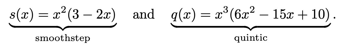

• The technique starts by computing (u′,v′) (same as used in Equation 6.1 and in Figure 6.9) by first multiplying the sample by the texture dimensions and adding 0.5. The integer parts are kept for later, and the fractions are stored in u′ and v′, which are in the range of [0, 1]. The (u′, v′) are then transformed as (tu, tv) = (q(u′), q(v′)), still in the range of [0, 1]. Finally, 0.5 is subtracted and the integer parts are added back in; the resulting u-coordinate is then divided by the texture width, and similarly for v. At this point, the new texture coordinates are used with the bilinear interpolation lookup provided by the GPU. Note that this method will give plateaus at each texel, which means that if the texels are located on a plane in RGB space, for example, then this type of interpolation will give a smooth, but still staircased, look, which may not always be desired.

Minification

To achieve this goal, either the pixel’s sampling frequency has to increase or the texture frequency has to decrease.

The basic idea behind all texture antialiasing algorithms is the same: to preprocess the texture and create data structures that will help compute a quick approximation of the effect of a set of texels on a pixel. For real-time work, these algorithms have the characteristic of using a fixed amount of time and resources for execution. In this way, a fixed number of samples are taken per pixel and combined to compute the effect of a (potentially huge) number of texels.

Mipmapping

Two important elements in forming high-quality mipmaps are good filtering and gamma correction. The common way to form a mipmap level is to take each 2 × 2 set of texels and average them to get the mip texel value.

For textures encoded in a nonlinear space (such as most color textures), ignoring gamma correction when filtering will modify the perceived brightness of the mipmap levels. As you get farther away from the object and the uncorrected mipmaps get used, the object can look darker overall, and contrast and details can also be affected.

Most APIs have support for sRGB textures, and so will generate mipmaps correctly in linear space and store the results in sRGB. When sRGB textures are accessed, their values are first converted to linear space so that magnification and minification are performed properly.

As mentioned earlier, some textures have a fundamentally nonlinear relationship to the final shaded color. Although this poses a problem for filtering in general, mipmap generation is particularly sensitive to this issue, since many hundred or thousands of pixels are being filtered. Specialized mipmap generation methods are often needed for the best results.

The basic process of accessing this structure while texturing is straightforward. A screen pixel encloses an area on the texture itself.The goal is to determine roughly how much of the texture influences the pixel. There are two common measures used to compute d (which OpenGL calls λ, and which is also known as the texture level of detail).

• One is to use the longer edge of the quadrilateral formed by the pixel’s cell to approximate the pixel’s coverage.
• Another is to use as a measure the largest absolute value of the four differentials

These gradient values are available to pixel shader programs using Shader Model 3.0 or newer. Since they are based on the differences between values in adjacent pixels,they are not accessible in sections of the pixel shader affected by dynamic flow control. For texture reads to be performed in such a section (e.g., inside a loop), the derivatives must be computed earlier. Note that since vertex shaders cannot access gradient information, the gradients or the level of detail need to be computed in the vertex shader itself and supplied to the GPU when using vertex texturing.

The (u, v, d) triplet is used to access the mipmap. The value d is analogous to a texture level, but instead of an integer value, d has the fractional value of the distance between levels. The texture level above and the level below the d location is sampled. The (u, v) location is used to retrieve a bilinearly interpolated sample from each of these two texture levels. The resulting sample is then linearly interpolated, depending on the distance from each texture level to d. This entire process is called trilinear interpolation and is performed per pixel.

One user control on the d-coordinate is the level of detail bias (LOD bias). This is a value added to d, and so it affects the relative perceived sharpness of a texture.

• The benefit of mipmapping is that, instead of trying to sum all the texels that affect a pixel individually, precombined sets of texels are accessed and interpolated. This process takes a fixed amount of time, no matter what the amount of minification.

Summed-Area Tables

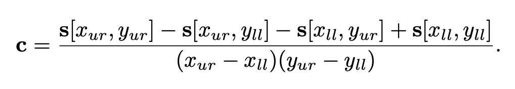
To use this method, one first creates an array that is the size of the texture but contains more bits of precision for the color stored. At each location in this array, one must compute and store the sum of all the corresponding texture’s texels in the rectangle formed by this location and texel (0, 0) (the origin). During texturing, the pixel cell’s projection onto the texture is bound by a rectangle. The summed-area table is then accessed to determine the average color of this rectangle, which is passed back as the texture’s color for the pixel.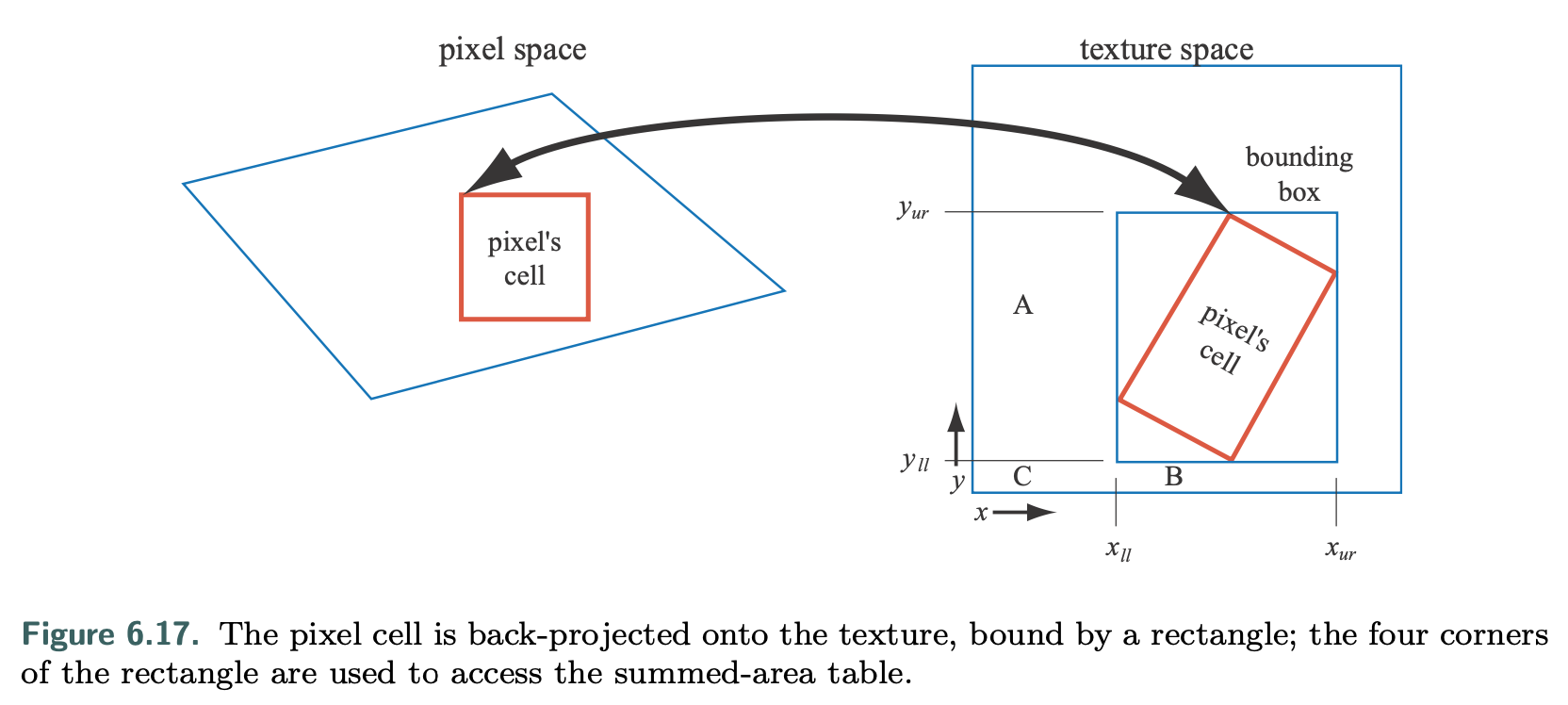

The summed-area table is an example of what are called anisotropic filtering algorithms. Such algorithms retrieve texel values over areas that are not square. However, SAT is able to do this most effectively in primarily horizontal and vertical directions. Note also that summed-area tables take at least two times as much memory for textures of size 16 × 16 or less, with more precision needed for larger textures. Summed area tables, which give higher quality at a reasonable overall memory cost, can be implemented on modern GPUs.

Unconstrained Anisotropic Filtering

For current graphics hardware, the most common method to further improve texture filtering is to reuse existing mipmap hardware.

The basic idea is that the pixel cell is back-projected, this quadrilateral (quad) on the texture is then sampled several times, and the samples are combined. As outlined above, each mipmap sample has a location and a squarish area associated with it. Instead of using a single mipmap sample to approximate this quad’s coverage, the algorithm uses several squares to cover the quad. The shorter side of the quad can be used to determine d (unlike in mipmapping, where the longer side is often used); this makes the averaged area smaller (and so less blurred) for each mipmap sample. The quad’s longer side is used to create a line of anisotropy parallel to the longer side and through the middle of the quad.

This scheme allows the line of anisotropy to run in any direction, and so does not have the limitations of summed-area tables. It also requires no more texture memory than mipmaps do, since it uses the mipmap algorithm to do its sampling.

Volume Textures

Using volume textures for surface texturing is extremely inefficient, since the vast majority of samples are not used.

Cube Maps

Another type of texture is the cube texture or cube map, which has six square tex- tures, each of which is associated with one face of a cube. A cube map is accessed with a three-component texture coordinate vector that specifies the direction of a ray pointing from the center of the cube outward. The point where the ray intersects the cube is found as follows.

Texture Representation

There are several ways to improve performance when handling many textures in an application. Texture compression is described in Section 6.2.6, while the focus of this section is on texture atlases, texture arrays, and bindless textures, all of which aim to avoid the costs of changing textures while rendering. In Sections 19.10.1 and 19.10.2, texture streaming and transcoding are described.

To be able to batch up as much work as possible for the GPU, it is generally preferred to change state as little as possible。

Texture Atlases

To that end, one may put several images into a single larger texture, called a texture atlas.

One difficulty with using an atlas is wrapping/repeat and mirror modes, which will not properly affect a subtexture but only the texture as a whole.

Another problem can occur when generating mipmaps for an atlas, where one subtexture can bleed into another. However, this can be avoided by generating the mipmap hierarchy for each subtexture separately before placing them into a large texture atlas and using power-of-two resolutions for the subtextures

Texture Arrays

A simpler solution to these issues is to use an API construction called texture ar- rays, which completely avoids any problems with mipmapping and repeat modes.

All subtextures in a texture array need to have the same dimensions, format, mipmap hierarchy, and MSAA settings. Like a texture atlas, setup is only done once for a texture array, and then any array element can be accessed using an index in the shader. This can be 5× faster than binding each subtexture.

Bindless Textures

Without bindless textures, a texture is bound to a specific texture unit using the API. One problem is the upper limit on the number of texture units, which complicates matters for the programmer.

The driver makes sure that the texture is resident on the GPU side. With bindless textures, there is no upper bound on the number of textures, because each texture is associated by just a 64-bit pointer, sometimes called a handle, to its data structure. These handles can be accessed in many different ways, e.g., through uniforms, through varying data, from other textures, or from a shader storage buffer object (SSBO).

The application needs to ensure that the textures are resident on the GPU side. Bindless textures avoid any type of binding cost in the driver, which makes rendering faster.

Texture Compression

One solution that directly attacks memory and bandwidth problems and caching concerns is fixed-rate texture compression. By having the GPU decode compressed textures on the fly, a texture can require less texture memory and so increase the effective cache size. At least as significant, such textures are more efficient to use, as they consume less memory bandwidth when accessed.

S3 developed a scheme called S3 Texture Compression (S3TC) , which was chosen as a standard for DirectX and called DXTC—in DirectX 10 it is called BC (for Block Compression).

It has the advantages of creating a compressed image that is fixed in size, has independently encoded pieces, and is simple (and therefore fast) to decode. Each compressed part of the image can be dealt with independently from the others. There are no shared lookup tables or other dependencies, which simplifies decoding.

S3TC/DXTC/BC Compression

There are seven variants of the DXTC/BC compression scheme, and they share some common properties.

• Encoding is done on 4 × 4 texel blocks, also called tiles.
• Each block is encoded separately.
• The encoding is based on interpolation.
• For each encoded quantity, two reference values (e.g., colors) are stored.
• An interpolation factor is saved for each of the 16 texels in the block. The compression comes from storing only two colors along with a short index value per pixel.

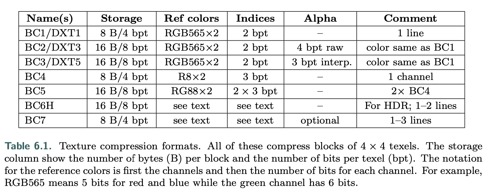
Note that “DXT” indicates the names in DirectX 9 and “BC” the names in DirectX 10 and beyond. As can be read in the table, BC1 has two 16-bit reference RGB values (5 bits red, 6 green, 5 blue), and each texel has a 2-bit interpolation factor to select from one of the reference values or two intermediate values.1 This represents a 6 : 1 texture compression ratio, compared to an uncompressed 24-bit RGB texture. BC2 encodes colors in the same way as BC1, but adds 4 bits per texel (bpt) for quantized (raw) alpha. For BC3, each block has RGB data encoded in the same way as a DXT1 block. In addition, alpha data are encoded using two 8-bit reference values and a per-texel 3-bit interpolation factor. Each texel can select either one of the reference alpha values or one of six intermediate values. BC4 has a single channel, encoded as alpha in BC3. BC5 contains two channels, where each is encoded as in BC3. BC6H is for high dynamic range (HDR) textures, where each texel initially has 16-bit floating point value per R, G, and B channel. This mode uses 16 bytes, which results in 8 bpt. It has one mode for a single line (similar to the techniques above) and another for two lines where each block can select from a small set of partitions. Two reference colors can also be delta-encoded for better precision and can also have different accuracy depending on which mode is being used. In BC7, each block can have between one and three lines and stores 8 bpt. The target is high-quality texture compression of 8-bit RGB and RGBA textures. It shares many properties with BC6H, but is a format for LDR textures, while BC6H is for HDR. Note that BC6H and BC7 are called BPTC_FLOAT and BPTC, respectively, in OpenGL. These compression techniques can be applied to cube or volume textures, as well as two-dimensional textures.

The main drawback of these compression schemes is that they are lossy. One of the problems with BC1–BC5 is that all the colors used for a block lie on a straight line in RGB space. For example, the colors red, green, and blue cannot be represented in a single block. BC6H and BC7 support more lines and so can provide higher quality.

For OpenGL ES, another compression algorithm, called Ericsson texture compression (ETC) was chosen for inclusion in the API. This scheme has the same features as S3TC, namely, fast decoding, random access, no indirect lookups, and fixed rate. It encodes a block of 4 × 4 texels into 64 bits, i.e., 4 bits per texel are used. Each 2 × 4 block (or 4 × 2, depending on which gives best quality) stores a base color. Each block also selects a set of four constants from a small static lookup table, and each texel in a block can select to add one of the values in this table. This modifies the luminance per pixel. The image quality is on par with DXTC.

In ETC2, included in OpenGL ES 3.0, unused bit combinations were used to add more modes to the original ETC algorithm. ETC2 added two new modes with four colors, derived differently, per block, and a final mode that is a plane in RGB space intended to handle smooth transitions.

Ericsson alpha compression (EAC) compresses an image with one component (e.g, alpha). This compression is like basic ETC compression but for only one component, and the resulting image stores 4 bits per texel. It can optionally be combined with ETC2, and in addition two EAC channels can be used to compress normals (more on this topic below). All of ETC1, ETC2, and EAC are part of the OpenGL 4.0 core profile, OpenGL ES 3.0, Vulkan, and Metal.

Normal Compression

Compressed formats that were designed for RGB colors usually do not work well for normal xyz data. This in itself results in a modest amount of compression, since only two components are stored, instead of three. Since most GPUs do not natively support three-component textures, this also avoids the possibility of wasting a component (or having to pack another quantity in the fourth component).

Further compression is usually achieved by storing the x- and y-components in a BC5/3Dc-format texture. Since the reference values for each block demarcate the minimum and maximum x- and y-component values, they can be seen as defining a bounding box on the xy-plane. The three-bit interpolation factors allow for the selection of eight values on each axis, so the bounding box is divided into an 8 × 8 grid of possible normals. Alternatively, two channels of EAC (for x and y) can be used, followed by computation of z as defined above.

On hardware that does not support the BC5/3Dc or the EAC format, a common fallback is to use a DXT5-format texture and store the two components in the green and alpha components (since those are stored with the highest precision). The other two components are unused.

Other Compression Formats

PVRTC is a texture compression format available on Imagination Technologies’ hardware called PowerVR, and its most widespread use is for iPhones and iPads.

Adaptive scalable texture compression (ASTC) is different in that it com- presses a block of n × m texels into 128 bits. The block size ranges from 4 × 4 up to 12 × 12, which results in different bit rates, starting as low as 0.89 bits per texel and going up to 8 bits per texel. ASTC uses a wide range of tricks for compact index representation, and the numbers of lines and endpoint encoding can be chosen per block. In addition, ASTC can handle anything from 1–4 channels per texture and both LDR and HDR textures. ASTC is part of OpenGL ES 3.2 and beyond.

All the texture compression schemes presented above are lossy, and when com- pressing a texture, one can spend different amounts of time on this process. This is often done as an offline preprocess and is stored for later use.

Decompression is extremely fast since it is done using fixed-function hardware. This difference is called data compression asymmetry, where compression can and does take a considerably longer time than decompression.

several methods that can improve the quality of the compressed textures

• For both textures containing colors and normal maps, it is recommended that the maps are authored with 16 bits per component.
• For color textures, one then performs a histogram renormalization (on these 16 bits), the effect of which is then inverted using a scale and bias constant (per texture) in the shader.
• Histogram normalization is a technique that spreads out the values used in an image to span the entire range, which effectively is a type of contrast enhancement.
• Using 16 bits per component makes sure that there are no unused slots in the histogram after renormalization, which reduces banding artifacts that many texture compression schemes may introduce.
• In addition, Kaplanyan recommends using a linear color space for the texture if 75% of the pixels are above 116/255, and otherwise storing the texture in sRGB.
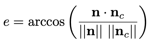
• For normal maps, he also notes that BC5/3Dc often compresses x independently from y, which means that the best normal is not always found. Instead, he proposes to use the following error metric for normals: where n is the original normal and nc is the same normal compressed, and then decompressed.

It should be noted that it is also possible to compress textures in a different color space, which can be used to speed up texture compression. A commonly used trans- form is RGB→YCoCg, where Y is a luminance term and Co and Cg are chrominance terms. The inverse transform is also inexpensive.

There is another reversible RGB→YCoCg transform. This means that it is possible to transform back and forth between, say, a 24-bit RGB color and the corresponding YCoCg representation without any loss.

Note that for textures that are dynamically created on the CPU, it may be better to compress the textures on the CPU as well. When textures are created through rendering on the GPU, it is usually best to compress the textures on the GPU as well.