Fresnel Reflectance
In Section 9.1 we discussed light-matter interaction from a high level. In Section 9.3, we covered the basic machinery for expressing these interactions mathematically: the BRDF and the reflectance equation. Now we are ready to start drilling down to specific phenomena, quantifying them so they can be used in shading models. We will start with reflection from a flat surface, first discussed in Section 9.1.3.
An object’s surface is an interface between the surrounding medium (typically air) and the object’s substance. The interaction of light with a planar interface between two substances follows the Fresnel equations developed by Augustin-Jean Fresnel (1788~1827). The Fresnel equations require a flat interface following the assumptions of geometrical optics. In other words, the surface is assumed to not have any irregularities between 1 light wavelength and 100 wavelengths in size. Irregularities smaller than this range have no effect on the light, and larger irregularities effectively tilt the surface but do not affect its local flatness.
Light incident on a flat surface splits into a reflected part and a refracted part. The direction of the reflected light (indicated by the vector $r_i$) forms the same angle ($\theta_i$) with the surface normal $n$ as the incoming direction $l$. The reflection vector $r_i$ can be computed from $n$ and $l$: \(r_i = 2(n \cdot l) n - l\)
The amount of light reflected (as a fraction of incoming light) is described by the Fresnel reflectance F, which depends on the incoming angle $\theta_i$.
As discussed in Section 9.1.3, reflection and refraction are affected by the refractive index of the two substances on either side of the plane. We will continue to use the notation from that discussion. The value $n_1$ is the refractive index of the substance “above” the interface, where incident and reflected light propagate, and $n_2$ is the refractive index of the substance “below” the interface, where the refracted light propagates. The Fresnel equations describe the dependence of $F$ on $\theta_i$, $n_1$, and $n_2$. Rather than present the equations themselves, which are somewhat complex, we will describe their important characteristics.
External Reflection
External reflection is the case where $n_1 < n_2$. In other words, the light originates on the side of the surface where the refractive index is lower. Most often, this side contains air, with a refractive index of approximately 1.003. We will assume $n_1= 1$ for simplicity. The opposite transition, from object to air, is called internal reflection and is discussed later in Section 9.5.3.
For a given substance, the Fresnel equations can be interpreted as defining a reflectance function $F(\theta_i)$, dependent only on incoming light angle. In principle, the value of $F(\theta_i)$ varies continuously over the visible spectrum. For rendering purposes its value is treated as an RGB vector. The function $F(\theta_i)$ has the following characteristics:
- When $\theta_i= 0^\circ$, with the light perpendicular to the surface $(l = n)$, $F(\theta_i)$ has a value that is a property of the substance. This value, $F_0$, can be thought of as the characteristic specular color of the substance. The case when $\theta_i= 0^\circ$ is called normal incidence.
- As $\theta_i$ increases and the light strikes the surface at increasingly glancing angles, the value of $F(\theta_i)$ will tend to increase, reaching a value of 1 for all frequencies (white) at $\theta_i= 90^\circ$.
Figure 9.20 shows the $F(\theta_i)$ function, visualized in several different ways, for several substances. The curves are highly nonlinear-they barely change until $\theta_i = 75^\circ$ or so, and then quickly go to 1. The increase from $F_0$ to 1 is mostly monotonic, though some substances (e.g., aluminum in Figure 9.20) have a slight dip just before going to white.
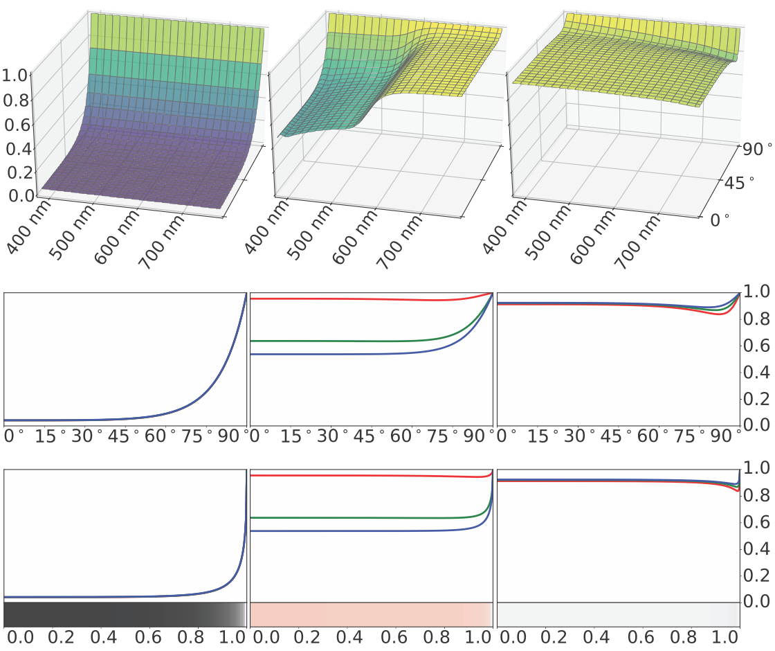
Figure 9.20. Fresnel reflectance $F$ for external reflection from three substances: glass, copper, and aluminum (from left to right). The top row has three-dimensional plots of $F$ as a function of wavelength and incidence angle. The second row shows the spectral value of $F$ for each incidence angle converted to RGB and plotted as separate curves for each color channel. The curves for glass coincide, as its Fresnel reflectance is colorless. In the third row, the R, G, and B curves are plotted against the sine of the incidence angle, to account for the foreshortening shown in Figure 9.21. The same x-axis is used for the strips in the bottom row, which show the RGB values as colors.
In the case of mirror reflection, the outgoing or view angle is the same as the incidence angle. This means that surfaces that are at a glancing angle to the incoming light-with values of $\theta_i$ close to $90^\circ$ -are also at a glancing angle to the eye. For this reason, the increase in reflectance is primarily seen at the edges of objects. Furthermore, the parts of the surface that have the strongest increase in reflectance are foreshortened from the camera’s perspective, so they occupy a relatively small number of pixels. To show the different parts of the Fresnel curve proportionally to their visual prominence, the Fresnel reflectance graphs and color bars in Figure 9.22 and the lower half of Figure 9.20 are plotted against $\sin(\theta_i)$ instead of directly against $\theta_i$. Figure 9.21 illustrates why $\sin(\theta_i)$ is an appropriate choice of axis for this purpose.
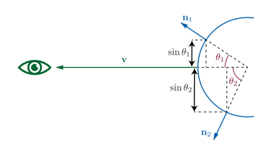
Figure 9.21. Surfaces tilted away from the eye are foreshortened. This foreshortening is consistent with projecting surface points according to the sine of the angle between $v$ and $n$ (for mirror reflection this is the same as the incidence angle). For this reason, Fresnel reflectance is plotted against the sine of the incidence angle in Figures 9.20 and 9.22.
From this point, we will typically use the notation $F(n, l)$ instead of $F(\theta_i)$ for the Fresnel function, to emphasize the vectors involved. Recall that $\theta_i$ is the angle between the vectors $n$ and $l$. When the Fresnel function is incorporated as part of a BRDF, a different vector is often substituted for the surface normal $n$. See Section 9.8 for details.
The increase in reflectance at glancing angles is often called the Fresnel effect in rendering publications (in other fields, the term has a different meaning relating to transmission of radio waves).
Besides their complexity, the Fresnel equations have other properties that makes their direct use in rendering difficult. They require refractive index values sampled over the visible spectrum, and these values may be complex numbers. The curves in Figure 9.20 suggest a simpler approach based on the characteristic specular color $F_0$. Schlick gives an approximation of Fresnel reflectance: \(F(n,l) \approx F_0+(1-F_0)(1-(n \cdot l)^+)^5\) This function is an RGB interpolation between white and $F_0$. Despite this simplicity, the approximation is reasonably accurate.
Figure 9.22 contains several substances that diverge from the Schlick curves, exhibiting noticeable “dips” just before going to white. In fact, the substances in the bottom row were chosen because they diverge from the Schlick approximation to an especially large extent. Even for these substances the resulting errors are quite subtle, as shown by the color bars at the bottom of each plot in the figure. In the rare cases where it is important to precisely capture the behavior of such materials, an alternative approximation given by Gulbrandsen can be used. This approximation can achieve a close match to the full Fresnel equations for metals, though it is more computationally expensive than Schlick’s. A simpler option is to modify Schlick’s approximation to allow for raising the final term to powers other than 5 (as in Equation 9.18). This would change the “sharpness” of the transition to white at $90^\circ$, which could result in a closer match. Lagarde summarizes the Fresnel equations and several approximations to them.
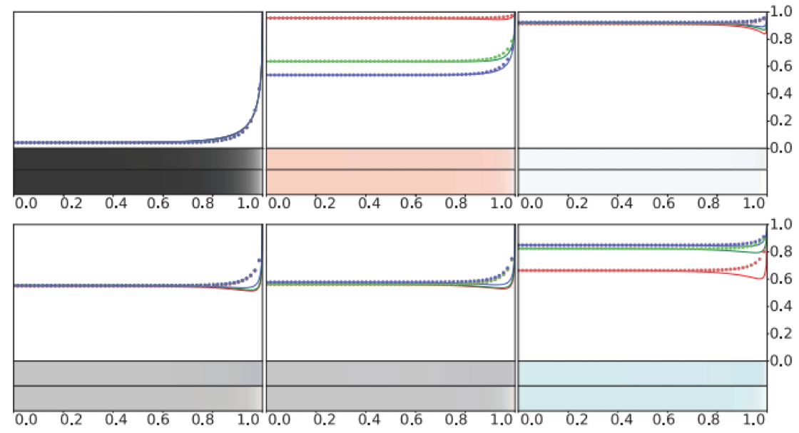
Figure 9.22. Schlick’s approximation to Fresnel reflectance compared to the correct values for external reflection from six substances. The top three substances are the same as in Figure 9.20: glass, copper, and aluminum (from left to right). The bottom three substances are chromium, iron, and zinc. Each substance has an RGB curve plot with solid lines showing the full Fresnel equations and dotted lines showing Schlick’s approximation. The upper color bar under each curve plot shows the result of the full Fresnel equations, and the lower color bar shows the result of Schlick’s approximation.
When using the Schlick approximation, $F_0$ is the only parameter that controls Fresnel reflectance. This is convenient since $F_0$ has a well-defined range of valid values in $[0, 1]$, is easy to set with standard color-picking interfaces, and can be textured using texture formats designed for colors. In addition, reference values for $F_0$ are available for many real-world materials. The refractive index can also be used to compute $F_0$. It is typical to assume that $n_1 = 1$, a close approximation for the refractive index of air, and use $n$ instead of $n_2$ to represent the refractive index of the object. This simplification gives the following equation: \(F_0 = (\frac{n-1}{n+1})^2\).
This equation works even with complex-valued refractive indices (such as those of metals) if the magnitude of the (complex) result is used. In cases where the refractive index varies significantly over the visible spectrum, computing an accurate RGB value for $F_0$ requires first computing $F_0$ at a dense sampling of wavelengths, and then converting the resulting spectral vector into RGB values using the methods described in Section 8.1.3.
In some applications a more general form of the Schlick approximation is used: \(F(n,l) \approx F_0 + (F_{90}-F_0)(1-(n \cdot l)^+)^{\frac{1}{p}}\)
This provides control over the color to which the Fresnel curve transitions at $90^\circ$, as well as the “sharpness” of the transition. The use of this more general form is typically motivated by a desire for increased artistic control, but it can also help match physical reality in some cases. As discussed above, modifying the power can lead to closer fits for certain materials. Also, setting $F_{90}$ to a color other than white can help match materials that are not described well by the Fresnel equations, such as surfaces covered in fine dust with grains the size of individual light wavelengths.
Typical Fresnel Reflectance Values
Substances are divided into three main groups with respect to their optical properties. There are dielectrics, which are insulators; metals, which are conductors; and semiconductors, which have properties somewhere in between dielectrics and metals.
Fresnel Reflectance Values for Dielectrics
Most materials encountered in daily life are dielectrics?glass, skin, wood, hair, leather, plastic, stone, and concrete, to name a few. Water is also a dielectric. This last may be surprising, since in daily life water is known to conduct electricity, but this conductivity is due to various impurities. Dielectrics have fairly low values for $F_0$?usually 0.06 or lower. This low reflectance at normal incidence makes the Fresnel effect especially visible for dielectrics. The optical properties of dielectrics rarely vary much over the visible spectrum, resulting in colorless reflectance values. The $F_0$ values for several common dielectrics are shown in Table 9.1. The values are scalar rather than RGB since the RGB channels do not differ significantly for these materials. For convenience, Table 9.1 includes linear values as well as 8-bit values encoded with the sRGB transfer function (the form that would typically be used in a texture-painting application).
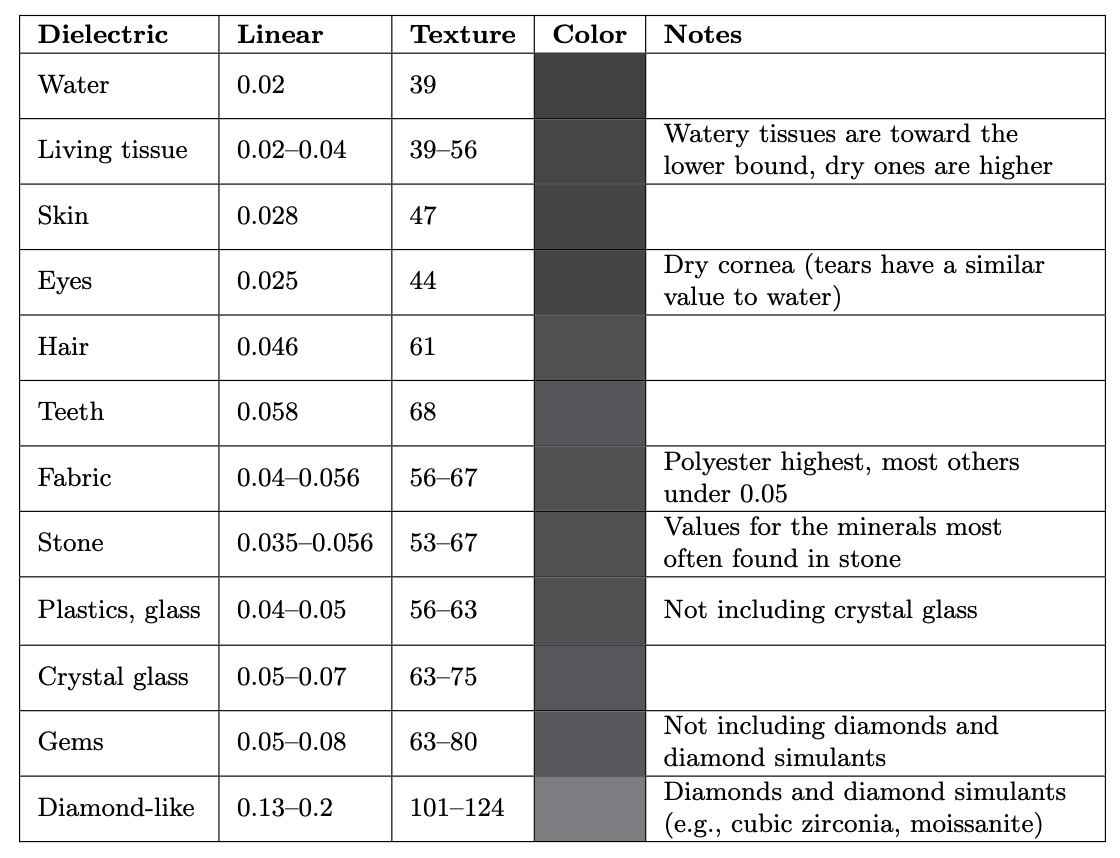
Table 9.1. Values of $F_0$ for external reflection from various dielectrics. Each value is given as a linear number, as a texture value (nonlinearly encoded 8-bit unsigned integer), and as a color swatch. If a range of values is given, then the color swatch is in the middle of the range.
Recall that these are specular colors. For example, gems often have vivid colors, but those result from absorption inside the substance and are unrelated to their Fresnel reflectance.
The $F_0$ values for other dielectrics can be inferred by looking at similar substances in the table. For unknown dielectrics, 0.04 is a reasonable default value, not too far off from most common materials.
Once the light is transmitted into the dielectric, it may be further scattered or absorbed. Models for this process are discussed in more detail in Section 9.9. If the material is transparent, the light will continue until it hits an object surface “from the inside,” which is detailed in Section 9.5.3.
Fresnel Reflectance Values for Metals
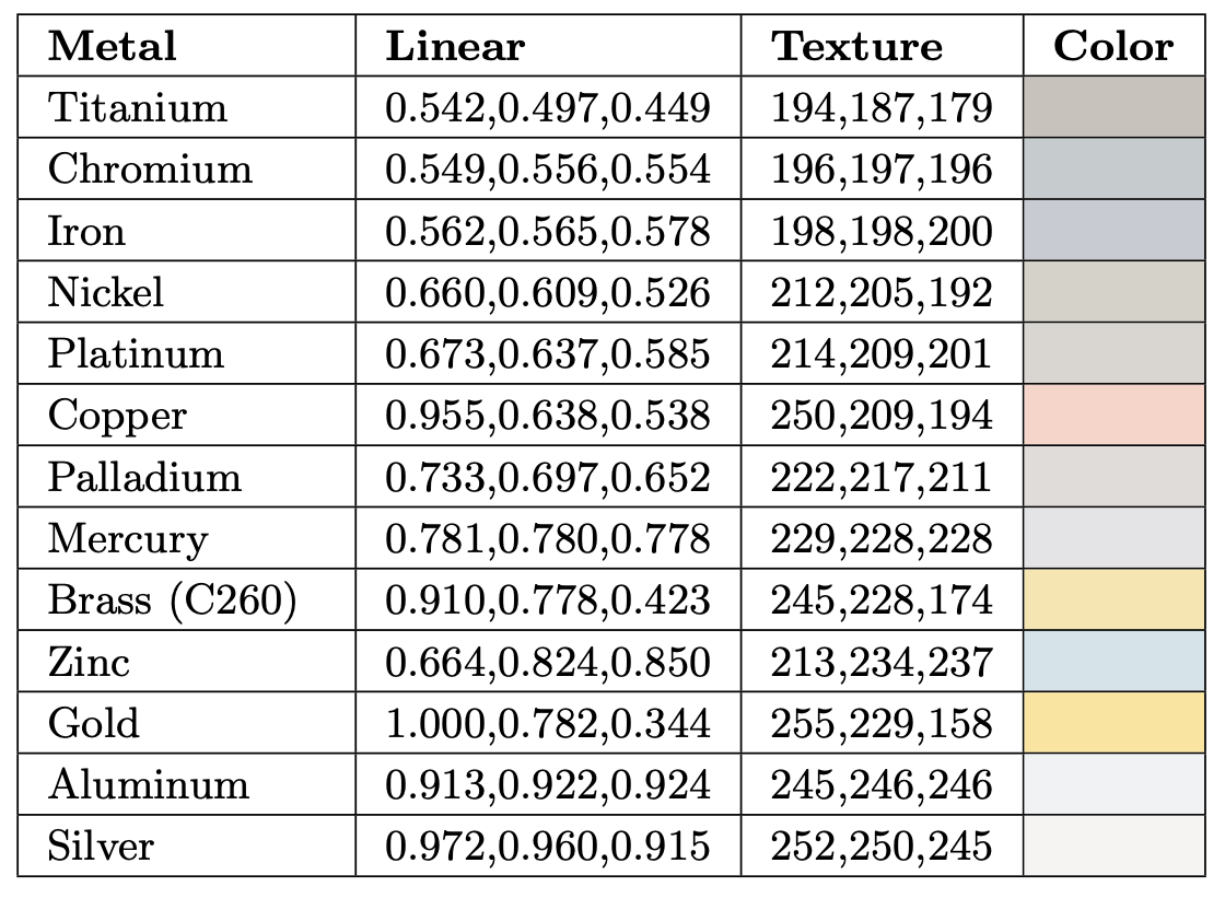
Table 9.2. Values of $F_0$ for external reflection from various metals (and one alloy), sorted in order of increasing lightness. The actual red value for gold is slightly outside the sRGB gamut. The value shown is after clamping.
Metals have high values of $F_0$?almost always 0.5 or above. Some metals have optical properties that vary over the visible spectrum, resulting in colored reflectance values. The $F_0$ values for several metals are shown in Table 9.2.
Similarly to Table 9.1, Table 9.2 has linear values as well as 8-bit sRGB-encoded values for texturing. However, here we give RGB values since many metals have colored Fresnel reflectance. These RGB values are defined using the sRGB (and Rec. 709) primaries and white point. Gold has a somewhat unusual $F_0$ value. It is the most strongly colored, with a red channel value slightly above 1 (it is just barely outside the sRGB/Rec. 709 gamut) and an especially low blue channel value (the only value in Table 9.2 significantly below 0.5). It is also one of the brightest metals, as can be seen by its position in the table, which is sorted in order of increasing lightness. Gold’s bright and strongly colored reflectance probably contributes to its unique cultural and economic significance throughout history.
Recall that metals immediately absorb any transmitted light, so they do not exhibit any subsurface scattering or transparency. All the visible color of a metal comes from $F_0$.
Fresnel Reflectance Values for Semiconductors
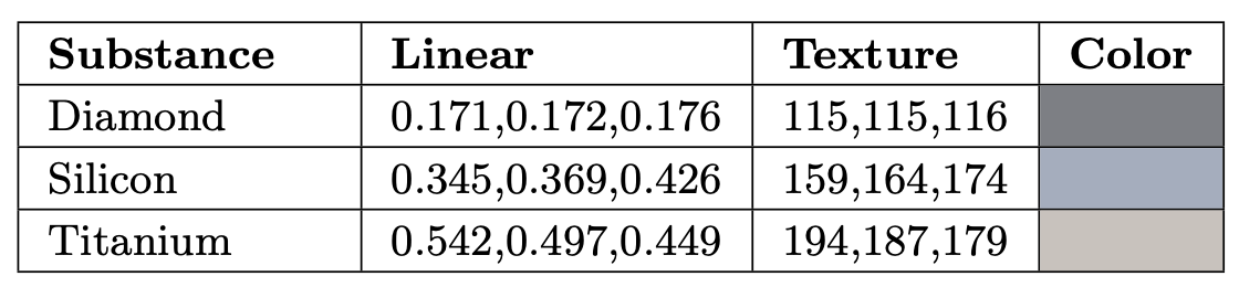
Table 9.3. The value of $F_0$ for a representative semiconductor (silicon in crystalline form) compared to a bright dielectric (diamond) and a dark metal (titanium).
As one would expect, semiconductors have $F_0$ values in between the brightest dielectrics and the darkest metals, as shown in Table 9.3. It is rare to need to render such substances in practice, since most rendered scenes are not littered with blocks of crystalline silicon. For practical purposes the range of $F_0$ values between 0.2 and 0.45 should be avoided unless you are purposely trying to model an exotic or unrealistic material.
Fresnel Reflectance Values in Water
In our discussion of external reflectance, we have assumed that the rendered surface is surrounded by air. If not, the reflectance will change, since it depends on the ratio between the refractive indices on both sides of the interface. If we can no longer assume that $n_1 = 1$, then we need to replace $n$ in Equation with the relative index of refraction, $n_1/n_2$. This yields the following, more general equation: \(F_0 = (\frac{n_1 - n_2}{n_1 + n_2})^2\).
Likely the most frequently encountered case where $n_1 \neq 1$ is when rendering underwater scenes. Since water’s refractive index is about 1.33 times higher than that of air, values of $F_0$ are different underwater. This effect is stronger for dielectrics than for metals, as can be seen in Table 9.4.
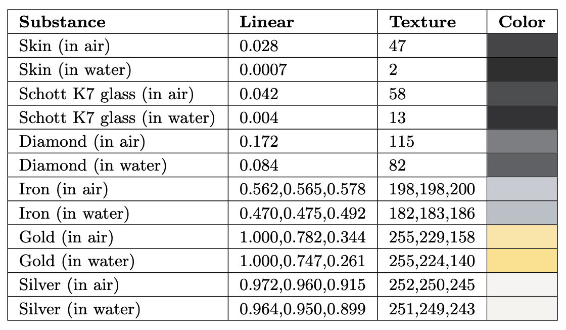
Table 9.4. A comparison between values of $F_0$ in air and in water, for various substances. As one would expect from inspecting Equation 9.19, dielectrics with refractive indices close to that of water are affected the most. In contrast, metals are barely affected.
Parameterizing Fresnel Values
An often-used parameterization combines the specular color $F_0$ and the diffuse color $\rho_{ss}$ (the diffuse color will be discussed further in Section 9.9). This parameterization takes advantage of the observation that metals have no diffuse color and that dielectrics have a restricted set of possible values for $F_0$ , and it includes an RGB surface color $\c_{surf}$ and a scalar parameter $m$, called “metallic” or “metalness.” If $m = 1$, then $F_0$ is set to $\c_{surf}$ and $\rho_{ss}$ is set to black. If $m = 0$, then $F_0$ is set to a dielectric value (either constant or controlled by an additional parameter) and $\rho_{ss}$ is set to $\c_{surf}$ .
The “metalness” parameter first appeared as part of an early shading model used at Brown University , and the parameterization in its current form was first used by Pixar for the film Wall-E . For the Disney principled shading model, used in Disney animation films from Wreck-It Ralph onward, Burley added an additional scalar “specular” parameter to control dielectric $F_0$ within a limited range . This form of the parameterization is used in the Unreal Engine , and the Frostbite engine uses a slightly different form with a larger range of possible $F_0$ values for dielectrics . The game Call of Duty: Infinite Warfare uses a variant that packs these metalness and specular parameters into a single value , to save memory.
For those rendering applications that use this metalness parameterization instead of using $F_0$ and $\rho_{ss}$ directly, the motivations include user convenience and saving texture or G-buffer storage. In the game Call of Duty: Infinite Warfare, this parameterization is used in an unusual way. Artists paint textures for $F_0$ and $\rho_{ss}$ , which are automatically converted to the metalness parameterization as a compression method.
Using metalness has some drawbacks. It cannot express some types of materials, such as coated dielectrics with tinted $F_0$ values. Artifacts can occur on the boundary between a metal and dielectric .
Another parameterization trick used by some real-time applications takes advantage of the fact that no materials have values of $F_0$ lower than 0.02, outside of special anti-reflective coatings. The trick is used to suppress specular highlights in surface areas that represent cavities or voids. Instead of using a separate specular occlusion texture, values of $F_0$ below 0.02 are used to “turn off” Fresnel edge brightening. This technique was first proposed by Schuler and is used in the Unreal and Frostbite engines.
Internal Reflection
Although external reflection is more frequently encountered in rendering, internal reflection is sometimes important as well. Internal reflection happens when $n_1 > n_2$. In other words, internal reflection occurs when light is traveling in the interior of a transparent object and encounters the object’s surface “from the inside.”
Snell’s law indicates that, for internal reflection, $\sin \theta_t> \sin \theta_i$. Since these values are both between $0^\circ$ and $90^\circ$, this relationship also implies $\theta_t > \theta_i$. In the case of external reflection the opposite is true. This difference is key to understanding how internal and external reflection differ. In external reflection, a valid (smaller) value of $\sin \theta_t$ exists for every possible value of $\sin \theta_i$ between 0 and 1. The same is not true for internal reflection. For values of $\theta_i$ greater than a critical angle $\theta_c$, Snell’s law implies that $\sin \theta_t> 1$, which is impossible. What happens in reality is that there is no $\theta_t$. When $\theta_i> \theta_c$, no transmission occurs, and all the incoming light is reflected. This phenomenon is known as total internal reflection.
The Fresnel equations are symmetrical, in the sense that the incoming and transmission vectors can be switched and the reflectance remains the same. In combination with Snell’s law, this symmetry implies that the $F(\theta_i)$ curve for internal reflection will resemble a “compressed” version of the curve for external reflection. The value of $F_0$ is the same for both cases, and the internal reflection curve reaches perfect reflectance at $\theta_c$ instead of at $90^\circ$. This is shown in Figure 9.24, which also shows that, on average, reflectance is higher in the case of internal reflection. For example, this is why air bubbles seen underwater have a highly reflective, silvery appearance.
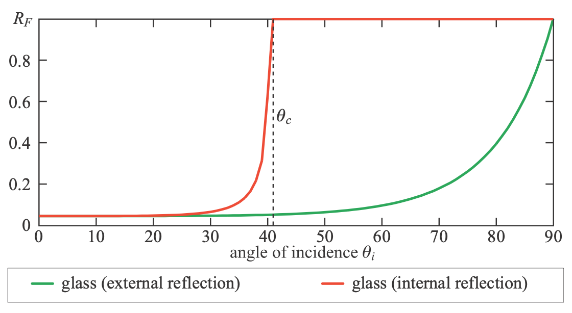
Figure 9.24. Comparison of internal and external reflectance curves at a glass-air interface. The internal reflectance curve goes to 1.0 at the critical angle $\theta_c$.
Internal reflection occurs only in dielectrics, as metals and semiconductors quickly absorb any light propagating inside them [285, 286]. Since dielectrics have real-valued refractive indices, computation of the critical angle from the refractive indices or from F0is straightforward: \(\sin \theta_c = \frac{n_2}{n_1} = \frac{1-\sqrt{F_0}}{1+\sqrt{F_0}}\).
The Schlick approximation is correct for external reflection. It can be used for internal reflection by substituting the transmission angle $\theta_t$ for $\theta_i$. If the transmission direction vector $t$ has been computed (e.g., for rendering refractions?see Section 14.5.2), it can be used for finding $\theta_t$. Otherwise Snell’s law could be used to compute $\theta_t$ from $\theta_i$, but that is expensive and requires the index of refraction, which may not be available.