Cloth Simulation | Intro to Physics-Based Animation

A Mass-Spring System

We could turn the mesh plane into a mass-spring system to simulate the cloth.

But first, we need to make raw mesh data into a data structure for simulation.

Topological Construction

• Raw mesh data:
  • Vertex List: 3d Vectors;
  • Triangle List: index triples.
• The key to topological construction is to sort triangle edge triples.
  • Each triple contains:
    • edge vertex index 0,
    • edge vertex index 1,
    • triangle index.
    • index 0 < index 1.
  • Sort the triples by the first two indices.
  • Then, we will find the repeated edges close to each other.
  • Remove the repeated edges and get the edge list. (The edge list is a list of pairs of vertex index 0 & 1.)
  • Construct Neighboring triangle list for bending using the repeated edges (triangle index).

Explicit Integration

Algorithm

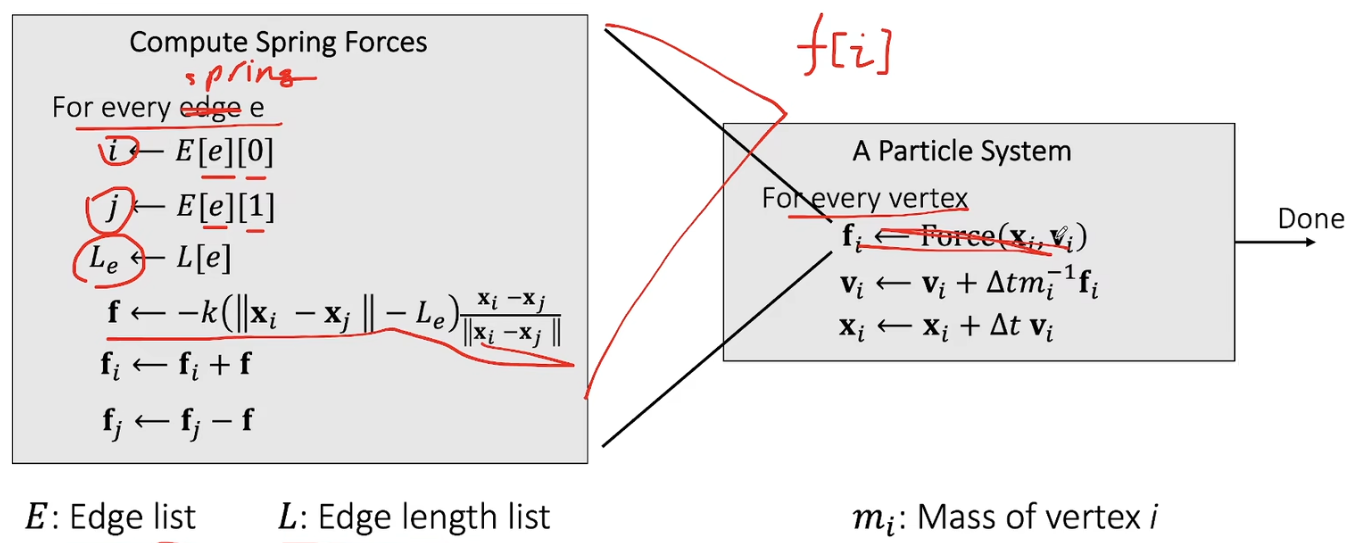
notice: the image isn’t correct. The force array should be calculated first, and then for every vertex we calculate velocity and position. { : .prompt-warning }

Explicit integration suffers from numerical instability caused by overshooting, when the stiffness $k$ and/or the time step $\Delta t$ is too large.

A naive solution is to use a small time step, but it is not efficient.

Implicit Integration

Implicit integration is a better solution to numerical instability. The idea is to integrate both velocity and position implicitly.

As the implicit method denots: \(\mathbf{v}^{[1]} = \mathbf{v}^{[0]} + \Delta t \mathbf{M}^{-1} \mathbf{f}^{[1]}, \quad \mathbf{x}^{[1]} = \mathbf{x}^{[0]} + \Delta t \mathbf{v}^{[1]}\) where $\mathbf{M}$ is the mass matrix, and $\mathbf{f}^{[1]}$ is the force array.

We can infer that: \(\mathbf{x}^{[1]} = \mathbf{x}^{[0]} + \Delta t \mathbf{v}^{[0]} + \Delta t^2 \mathbf{M}^{-1} \mathbf{f}^{[1]}, \quad \mathbf{v}^{[1]} = (\mathbf{x}^{[1]} - \mathbf{x}^{[0]})/\Delta t\)

Assuming that $\mathbf{f}$ is holonomic, i.e., depends only on $\mathbf{x}$, our goal is to solve the following equation: \(\mathbf{x}^{[1]} = \mathbf{x}^{[0]} + \Delta t \mathbf{v}^{[0]} + \Delta t^2 \mathbf{M}^{-1} \mathbf{f}(\mathbf{x}^{[1]})\)

The problem here is the nonlinearity of the equation (the force).

Let’s transform this equation into an optimization problem: \(\mathbf{x}^{[1]} = \argmin F(\mathbf{x}) \quad for \quad F(\mathbf{x}) = \frac{1}{2\Delta t^2}\vert\vert\mathbf{x} - \mathbf{x}^{[0]} - \Delta t \mathbf{v}^{[0]}\vert\vert^2_{\mathbf{M}} + E(\mathbf{x}),\quad where \quad \vert\vert\mathbf{x}\vert\vert_{\mathbf{M}}^2 = \mathbf{x}^T\mathbf{M}\mathbf{x}\) where the mass matrix $\mathbf{M}$ is often a diagonal matrix, and the energy $E(\mathbf{x})$ is the sum of all the energy of the whole system, i.e., $\frac{\partial E}{\partial \mathbf{x}} = \mathbf{f}(\mathbf{x})$. $\mathbf{x}$ is the position array with $\mathbf{x} \in \mathbb{R}^{3n}$ and $\mathbf{M} \in \mathbb{R}^{3n\times 3n}$.

It needs to denote that this transformation is not always correct since only conservative forces can be derived from potential energy. { : .prompt-warning }

This is because: \(\nabla F(\mathbf{x}^{[1]}) = \frac{1}{\Delta t^2}\mathbf{M}(\mathbf{x}^{[1]} - \mathbf{x}^{[0]} - \Delta t \mathbf{v}^{[0]}) - \mathbf{f}(\mathbf{x}^{[1]}) = 0\) which is equivalent to original equation.

Newton-Raphson Method

The Newton-Raphson method is a good choice to solve the optimization problem. It requires the Lipschitz continuity of the optimize function, which is often satisfied in practice.

Given a current $\mathbf{x}^{(k)}$, we approximate our goal by:

\(0 = F'(\mathbf{x}) \approx F'(\mathbf{x}^{(k)}) + F''(\mathbf{x}^{(k)})(\mathbf{x}- \mathbf{x}^{(k)})\) where $F’(\mathbf{x})$ is the gradient of $F(\mathbf{x})$, and $F’’(\mathbf{x})$ is the Hessian matrix of $F(\mathbf{x})$.

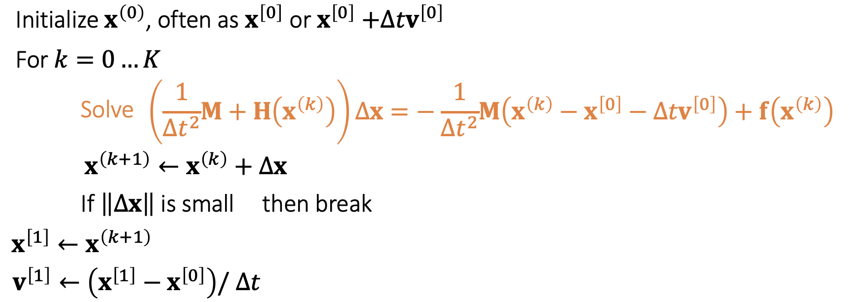
Algorithm below:

\(Initialize \mathbf{x}^{(0)}\) \(for\quad k = 0, 1, 2, ... K\quad do\) \(\Delta \mathbf{x} = -F''(\mathbf{x}^{(k)})^{-1}F'(\mathbf{x}^{(k)})\) \(\mathbf{x}^{(k+1)} = \mathbf{x}^{(k)} + \Delta \mathbf{x}\) \(if \vert\vert\Delta \mathbf{x}\vert\vert < \epsilon \quad then \quad break\)

Newton’s method finds an extremum, but it can be a minimum or maximum. We can use second-order information to determine the type of extremum.

Now we can apply the Newton-Raphson method to solve our problem.

\[\nabla F(\mathbf{x}^{(k)}) = \frac{1}{\Delta t^2}\mathbf{M}(\mathbf{x}^{(k)} - \mathbf{x}^{[0]} - \Delta t \mathbf{v}^{[0]}) - \mathbf{f}(\mathbf{x}^{(k)}),\quad \frac{\partial^2 F(\mathbf{x}^{(k)})}{\partial \mathbf{x}^2}= \frac{1}{\Delta t^2}\mathbf{M} - \mathbf{H}(\mathbf{x}^{(k)})\]

Algorithm below:

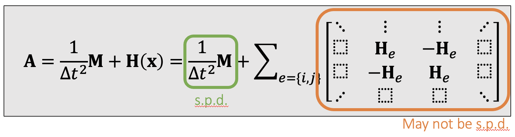
On Hessian Matrix of Mass-Spring System

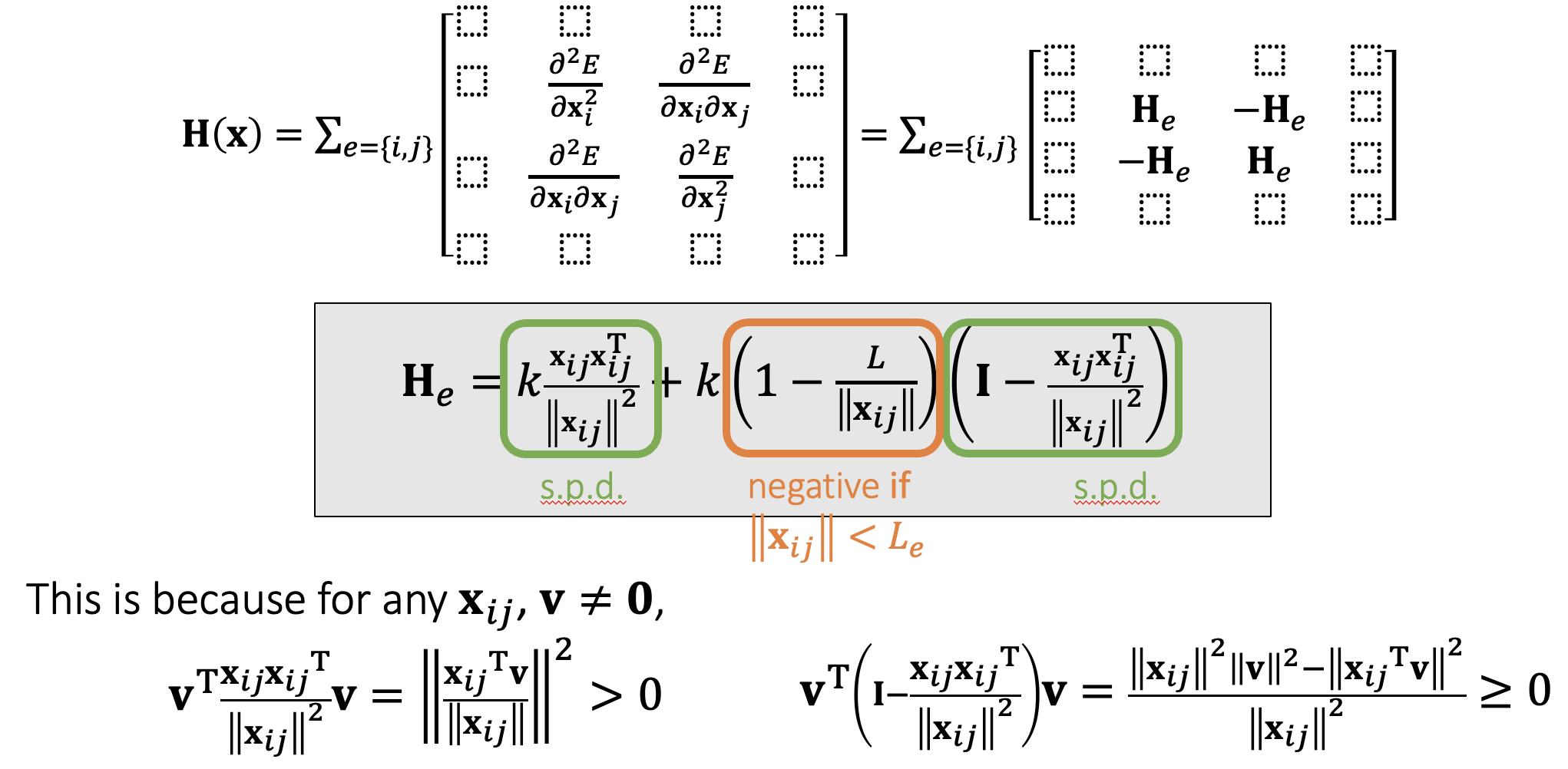
When a spring is stretched, $\mathbf{H}_e$ is s.p.d.; but when it’s compressed, $\mathbf{H}_e$ may not be s.p.d. As a result, $\mathbf{H(x),A}$ may not be s.p.d. either.

.

As before, if $\frac{\partial^2F}{\partial\mathbf{x}^2}$ is positive definite everywhere, $\mathbf{F(x)}$ has no maximum but only one minimum. This is a sufficient but not necessary condition.

When a spring is compressed, the spring Hessian may not be positive definite. This means there can be multiple local minima (outcomes). This issue occurs only in 2D and 3D. { : .prompt-tip }

Enforcement of Positive Definiteness

The enforcement is a must when considering the workability of solver. some linear solvers can fail to work if the matrix is not positive definite.

• One solution is to simply drop the ending term when the spring is compressed.
• Choi and Ko. 2002. Stable But Responive Cloth. TOG (SIGGRAPH)

Linear Solvers - Summary

• Direct Solvers (LU, LDLT, Cholesky, …)
  • One shot, expensive but worthy if you need exact solutions.
  • Little restriction on 𝐀
  • Mostly suitable on CPUs
• Iterative Solvers
  • Expensive to solve exactly, but controllable
  • Convergence restriction on 𝐀, typically positive definiteness
  • Suitable on both CPUs and GPUs
  • Easy to implement
  • Accelerable: Chebyshev, Nesterov, Conjugate Gradient…

Bending and Locking Issues

A Co-Rotational Method